Complex numbers
One of the fundamental ingredients of quantum information science (and, indeed, of quantum physics in general) is the notion of complex numbers.
It would be disingenuous to expect that a few paragraphs would suffice to make the reader sufficiently familiar with subject, but we try our best here to give a speedy overview of the core principles, and end with some exercises that can be a helpful indicator of which things you might want to read up on elsewhere.
The “classical” way of arriving at complex numbers is as follows: start with the natural numbers \mathbb{N}=\{0,1,2,\ldots\}, which we can add; if we want to be able to invert addition (i.e. subtract), then we end up with the integers \mathbb{Z}=\{\ldots,-2,-1,0,1,2,\ldots\}, which we can multiply; if we want to be able to invert multiplication (i.e. divide), then we end up with the rationals \mathbb{Q}=\{\frac{p}{q}\mid p,q\in\mathbb{Z}\}.
In this process of “closure under more and more binary operations”, we have passed from a monoid, to a group, to a field.
Algebraically, then, we seem to be done: we can do all the addition and multiplication that we like, and we can invert it whenever it makes sense to do so (e.g. we can divide, as long as it’s not by 0).
But there are lots of numbers that turn up in geometry that are not rational, such as \sqrt{2}\approx1.414, \pi\approx3.14, and e\approx2.718.
To include all of these (and simultaneously make sense of things like infinite sums, and limits), we must do some real analysis — something which we won’t touch upon here — to end up with the real numbers \mathbb{R}.
These form a field, just like the rationals, but now we don’t have any “gaps” in our number line.
So what’s left to do?
Well the reals have one big problem: they are not algebraically closed.
That is, there exist polynomials with no roots, i.e. equations of the form a_nx^n+a_{n-1}x^{n-1}+\ldots+a_1x+a_0=0 (where the a_i are real numbers) that have no solutions.
Somehow the most fundamental such example is the equation x^2+1=0, which has no solutions, because the square of any real number must be non-negative, and so \sqrt{-1}\not\in\mathbb{R}.
It turns out that if we just throw in this one extra number i\coloneqq\sqrt{-1} to \mathbb{R} then we can solve any polynomial — a theorem so important that it’s known as the fundamental theorem of algebra.
We call the result of doing this the complex numbers, and denote them by \mathbb{C}.
This gives us an algebraic way of understanding what a complex number is: it is a real number x plus an imaginary number iy (where y\in\mathbb{R})
That is, every complex number x+iy simply corresponds to a pair of real numbers (x,y).
So now we can think geometrically!
We imagine the complex numbers \mathbb{C} as the 2-dimensional Euclidean space \mathbb{R}^2, where the x-axis corresponds to the real part of a complex number, and the y-axis to the imaginary part.
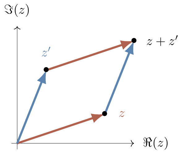
This really is a geometric way of thinking, since now addition (and subtraction) of complex numbers (which is defined by adding their real and imaginary parts separately) is given by vector addition, as shown in Figure 0.1.
But what about multiplication and division?
Following the rules of the game, we can figure out what the product of two complex numbers is by treating the imaginary number i as a “formal variable”, i.e. pretending it’s just a variable in some polynomial, and then remembering that i=\sqrt{-1} at the very end:
\begin{aligned}
(x+iy)(x'+iy')
&= xx'+ixy'+iyx'+i^2yy'
\\&= xx'+ixy'+iyx'-yy'
\\&= xx'-yy'+i(xy'+yx').
\end{aligned}
Division works similarly — the most simple example of inverting a complex number x+iy makes sense whenever x and y are both non-zero, since then we can use the trick of “multiplying by 1”:
\begin{aligned}
\frac{1}{x+iy}
&= \frac{1}{x+iy}\frac{x-iy}{x-iy}
\\&= \frac{x-iy}{x^2+y^2}
\\&= \frac{x}{x^2+y^2}-i\frac{y}{x^2+y^2}
\end{aligned}
This other complex number x-iy that we used is somehow special because it is exactly the thing we needed to make the denominator real, so we give it a name: the complex conjugate of a complex number z=x+iy is the complex number z^\star\coloneqq x-iy.
Geometrically, this is just the reflection of the vector (x,y)\in\mathbb{R}^2 in the x-axis.
The product zz^\star=x^2+y^2 is also important: you might recognise (from Pythagoras’ theorem) that \sqrt{x^2+y^2} is exactly the length of the vector (x,y), and so we call the real number |z|\coloneqq\sqrt{zz^\star} the modulus (or magnitude, norm, or absolute value).
Note then that we can simply write 1/z=z^\star/|z|^2.
Now things are looking somewhat nice, but the story isn’t complete.
We have a good geometric intuition for what a complex number is (a vector in \mathbb{R}^2) and how to add them (vector addition), as well as what the complex conjugate and the modulus mean (reflection in the x-axis, and the length of the vector, respectively); but what about multiplication and division?
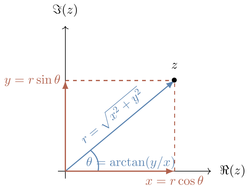
To understand these we need to switch from our rectangular coordinates z=x+iy to polar coordinates — instead of describing a point z in \mathbb{R}^2 as “x units left/right and y units up/down”, we describe it as “r units from the origin, at an angle of \theta radians”.
We already know, given (x,y)\in\mathbb{R}^2, how to calculate its distance r from the origin, since this is exactly the length of the vector: r=|(x,y)|=\sqrt{x^2+y^2}.
But what about the angle?
Some trigonometry tells us that \theta=\arctan(y/x), so we now know how to convert rectangular to polar coordinates:
x+iy = (x,y)
\longmapsto (r,\theta) \coloneqq (\sqrt{x^2+y^2},\arctan(y/x)).
It would be nice to know how to go in the other direction though, but this can also be solved with some trigonometry:
(r,\theta)
\longmapsto (r\cos\theta,r\sin\theta).
Great!
… but what’s the point of polar coordinates?
Well, it turns out that they give us a geometric way of understanding multiplication: you can show that (r,\theta) multiplied by (r',\theta') is exactly (rr',\theta+\theta'), which says that multiplication by a complex number (r,\theta) is exactly a scaling by a factor of r and a rotation by \theta.
This means that we can also easily find the multiplicative inverse of (r,\theta), since it’s just (1/r,-\theta).
Finally, complex conjugation just means switching the sign of the angle: (r,\theta)^\star=(r,-\theta).
There is one last ingredient that we should mention, which is the thing that really solidifies the relation between rectangular and polar coordinates.
We know that rectangular coordinates (x,y) can be written as x+iy, so is there some more algebraic way of writing polar coordinates (r,\theta)?
Then we can avoid any ambiguity that might arise from using pairs of numbers — if I tell you that I’m thinking of the complex number z=(0.3,2), do I mean the point 0.3+2i, or the point that is distance r from the origin at an angle of 2 radians?
Given polar coordinates (r,\theta), we know that this is equal to (r\cos\theta,r\sin\theta) in rectangular coordinates.
For simplicity, let’s first consider the case where r=1.
Then we can write (1,\theta) as \cos\theta+i\sin\theta.
Using the Taylor series of \sin and \cos, we can rewrite this as
\begin{aligned}
\cos\theta+i\sin\theta
&= \left(
1-\frac{\theta^2}{2!}+\frac{\theta^4}{4!}-\ldots
\right) + i\left(
\theta-\frac{\theta^3}{3!}+\frac{\theta^5}{5!}-\ldots
\right)
\\&= 1+i\theta-\frac{\theta^2}{2!}-i\frac{\theta^3}{3!}+\frac{\theta^4}{4!}+i\frac{\theta^5}{5!}-\ldots
\\&= 1+i\theta+\frac{i^2\theta^2}{2!}+\frac{i^3\theta^3}{3!}+\frac{i^4\theta^4}{4!}+\frac{i^5\theta^5}{5!}+\ldots
\\&= \exp(i\theta)
\end{aligned}
where at the very end we use the Taylor expansion of the exponential function \exp(x)=e^x.
We have just “proved” one of the most remarkable formulas in mathematics: Euler’s formula
e^{i\theta} = \cos\theta+i\sin\theta
(a special case of which gives the famous equation e^{i\pi}+1=0, uniting five fundamental constants: 0, 1, i, e, and \pi).
In summary then, we have two beautiful ways of expressing a complex number z\in\mathbb{C}, in either its rectangular/planar form or its polar/Euler form:
z = x+iy = re^{i\theta}.
Addition and subtraction are most neatly expressed in the planar form x+iy, and multiplication and division are most neatly expressed in the polar form re^{i\theta}; complex conjugation looks nice and tidy in both.
We know how to perform addition, multiplication, inversion (which is a special case of division), and complex conjugation on complex numbers in planar form, but we’ve only described how to do the last three of these in polar form: we haven’t said how to write re^{i\theta}+r'e^{i\theta'} as se^{i\varphi} for some s and \varphi.
This is because it is very messy looking:
\begin{aligned}
s
&= \sqrt{r^2+(r')^2+2rr'\cos(\theta'-\theta)}
\\\varphi
&= \theta+\operatorname{atan2}\big(r'\sin(\theta'-\theta),r+r'\cos(\theta'-\theta)\big)
\end{aligned}
and where \operatorname{atan2} is the 2-argument arctangent function.
You do not need to know everything about this whole story of algebraically closed fields and so on, but it helps to know the basics, so here are some exercises that should help you to become more familiar.
- The set \mathbb{Q} of rational numbers and the set \mathbb{R} of real numbers are both fields, but the set \mathbb{Z} of integers is not. Why not?
- Look up the formal statement of the fundamental theorem of algebra.
- Evaluate each of the following quantities:
1+e^{-i\pi},
\quad
|1+i|,
\quad
(1+i)^{42},
\quad
\sqrt{i},
\quad
2^i,
\quad
i^i.
- Here is a simple “proof” that +1=-1:
1=\sqrt{1}=\sqrt{(-1)(-1)}=\sqrt{-1}\sqrt{-1}=i^2=-1.
What is wrong with it?
- Prove that, for any two complex numbers w,z\in\mathbb{C}, we always have the inequality
|z-w| \geqslant|z|-|w|.
- Using the fact that e^{3i\theta}=(e^{i\theta})^3, derive a formula for \cos3\theta in terms of \cos\theta and \sin\theta.