The classical repetition code
We have now essentially met all the concepts of quantum error correction, but everything has been phrased in terms of correctable isometries.
Now we need to repeat much the same information from a slightly different perspective, including a brief detour to introduce some concepts and methods from the classical theory of error correction.
Even though quantum problems often require novel solutions, it is always a good idea to look at the classical world to see if there is anything equivalent there, and, if so, how people deal with it.
In this particular case, once we have digitised quantum errors, we can see that quantum decoherence is a bit like classical noise (i.e. bit-flips), except that we have two types of errors: these classical bit-flips, and then the purely quantum phase-flips.
But there’s one key thing that we know relating these two types of errors, namely that phase-flips can be turned into bit-flips by sandwiching then between Hadamard transforms:
HZH = X.
This opens up the possibility of adopting classical techniques of error correction to the quantum case.
There is a vast body of knowledge out there about classical error-correcting codes, and we can only scratch the surface here.
Suppose you want to send a k-bit message across a noisy channel.
If you choose to send the message directly, some bits may be flipped, and a different message will likely arrive with a certain number of errors.
Let’s suppose that the transmission channel flips each bit in transit with some fixed probability p.
If this error rate is considered too high, then it can be decreased by introducing some redundancy.
For example, we could encode each bit into three bits:
\begin{aligned}
0
&\longmapsto 000
\\1
&\longmapsto 111.
\end{aligned}
These two binary strings, 000 and 111, are called codewords.
Beforehand, Alice and Bob agree that, from now on, each time you want to send a logical 0, you will encode it as 000, and each time you want to send a logical 1, you will encode it as 111.
Here’s an example.
Say that Alice wants to send the message 1011.
She first encodes it as the string
111\,000\,111\,111
and then sends it to Bob over the noisy channel.
Note that she is now not sending just four, but instead twelve physical bits.
This is more costly (in terms of time or energy, or maybe even money), but might be worth it to ensure a more reliable transmission.
Let’s say that Bob then receives the message
110\,010\,101\,100.
Clearly some errors have occurred!
In fact, even Bob knows this, because he expects to receive 3-bit chunks of either all 0s or all 1s.
He uses the “majority vote” decoding method:
- 110 is decoded as 1
- 010 is decoded as 0
- 101 is decoded as 1
- 100 is decoded as 0.
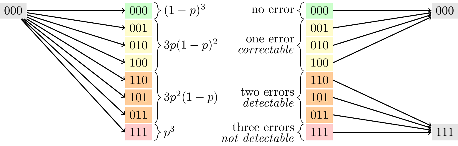
As we can see, if a triplet contains either zero or one errors then the decoding returns the correct bit value, otherwise it errs.
In our example, the first three triplets are correctly decoded, but the fourth suffered two errors and is thus wrongly decoded as 0.
This whole process can be represented as
1011
\overset{\text{encoding}}{\longmapsto} 111\,000\,111\,111
\overset{\text{noise}}{\longmapsto} 110\,010\,101\,100
\overset{\text{decoding}}{\longmapsto} 1010.
The noisy channel flipped 5 out of the 12 physical bits, and the whole encoding–decoding process reduced this down to only one logical error.
We can make a simple estimate on how good this scheme will be.
Assuming that the errors are independent then, for any given triplet,
\begin{cases}
\text{no errors}
& \text{probability }(1-p)^3
\\\text{1 error}
& \text{probability }3p(1-p)^2
\\\text{2 errors}
& \text{probability }3p^2(1-p)
\\\text{3 errors}
& \text{probability }p^3.
\end{cases}
More succinctly, the probability that n errors occur is
{3\choose n}p^n(1-p)^{3-n}
where \binom{m}{n}=m!/(n!(m-n)!) is the binomial coefficient.
Given that the scheme decodes correctly exactly when we have at most one error, the net probability of errors is just the probability that either two or three errors occur, which is
3p^2(1-p) + p^3.
This means that our encoding–decoding scheme actually lowers the probability of error if and only if
3p^2(1-p) + p^3
< \frac{1}{2}
i.e. when p<1/2.
This important number is known as the error threshold of the code, and is a good judge of how useful a code actually is.
When p is really small, we can basically ignore the p^3 term, since it is even smaller still, and claim that the error probability is reduced from p to roughly 3p^2.
In this example, we can see that if one or two errors occur, then the resulting bit string will no longer be a valid codeword, which makes the error detectable.
For example, if the bit string 101 appears in our message, then we know that some error must have occurred, because 101 is not a codeword, so we never would have sent it.
We can’t be certain which error has occurred, since it could have been a single bit-flip on 111 (more likely) or a double bit-flip on 000 (less likely), but we know for sure that one of these two went wrong.
In the worst case scenario, where three bit-flips happen, the error will be undetectable: it will turn 000 into 111 (and vice versa).
This results in what is known as a logical error, where the corrupted string is also a codeword, leaving us with no indication that anything has gone wrong.
Below a certain error threshold, the three-bit code improves the reliability of the information transfer.
This simple repetition code encoded one bit into three bits, and corrected up to one error.
In general, there are classical codes that can encode k bits into n bits and correct up to r errors.
One more important number that we need is the distance of such an encoding, which is defined to be the minimum number of errors that can pass undetected (or, equivalently, the minimum Hamming distance between two codewords).
More generally, the distance d relates to the number of errors t that a code can correct by d=2t+1, or, equivalently, t=\lfloor d/2\rfloor.
Looking back again at Figure 13.5, we see that if exactly one or two errors occur in our three-bit code then we can detect that an error has occurred, since we will have a string where not all of the bits are the same, which means that it is definitely not one of our code words.
However, if three errors occur then the errors are not only impossible to correct, but they are also impossible to detect.
So the code that we have described has n=3, k=1, and d=3.
A code that encodes k bits into n bits and has a distance of d is called an [n,k,d] code.
The rate of an [n,k,d] code is defined to be R=k/n.
In an [n,k,d] code, the encoder divides the message into chunks of k bits and encodes each k-bit string into a pre-determined n-bit codeword.
There are 2^k distinct codewords among all 2^n binary strings of length n.
The recipient then applies the decoder, which takes chunks of n bits, looks for the nearest codeword (in terms of Hamming distance), and then decodes the n-bit string into that k-bit codeword.
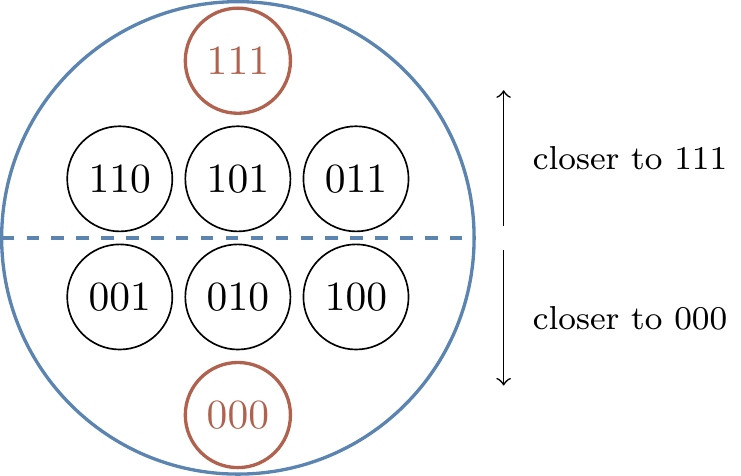
For example, in our 3-bit repetition code, we have the two codewords 000 and 111, among all eight binary strings of length 3, as shown in Figure 13.6.