Quantum Fourier transform
In Section 10.8 we constructed a circuit to perform phase estimation of an unknown rational phase \varphi=2\pi m/2^n.
The circuit, as per usual, was split into three parts: first some Hadamard gates, then a modified controlled-U gate, and finally some undefined gate FT^\dagger.
Following our usual credo, this last gate should look something like a Hadamard, and we shall see that it is indeed related.
This gate turns out to be pretty foundational, and turns up all over the place, so it’s worth taking some time to talk about it in more detail.
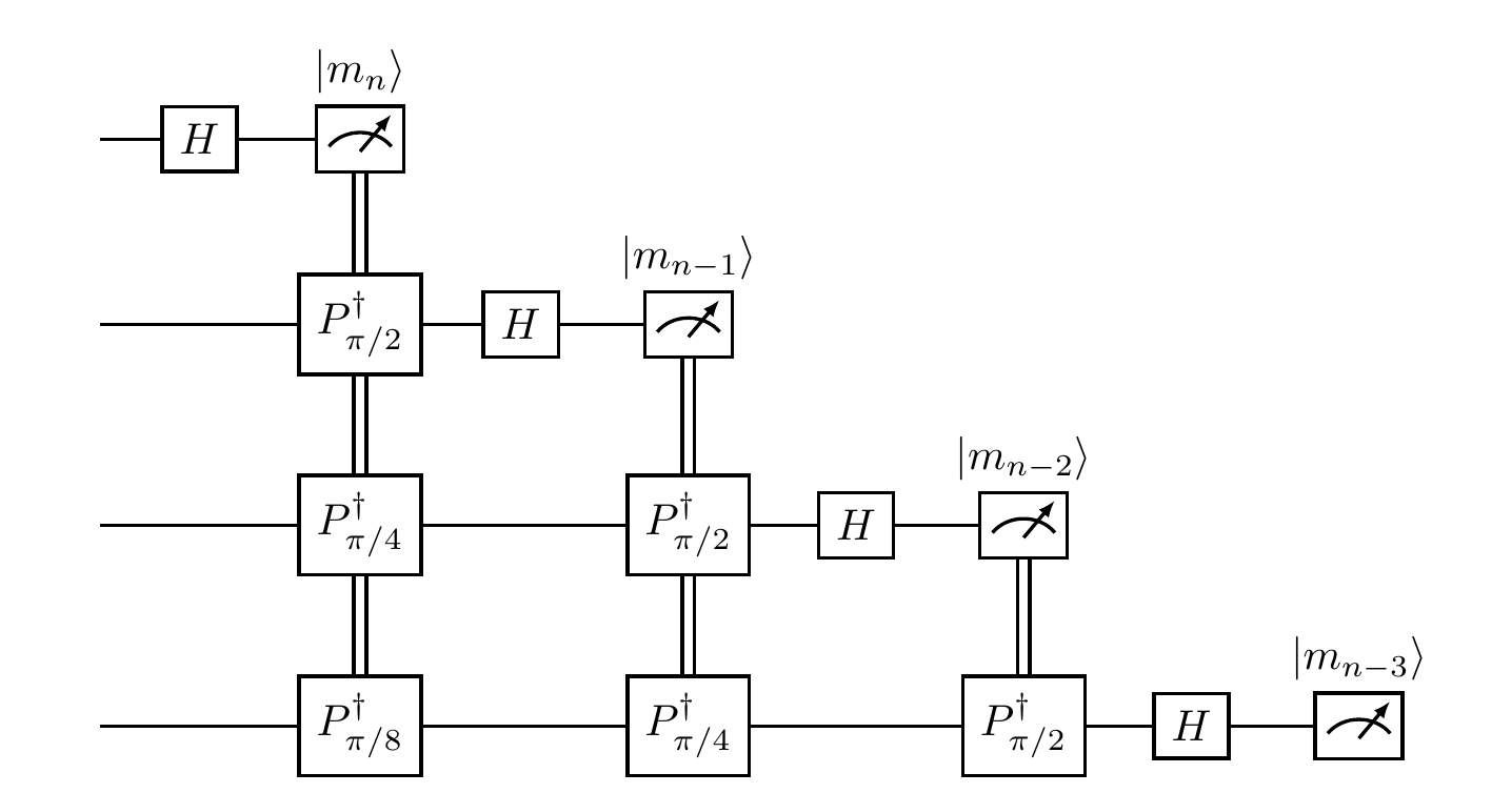
If we look back at what we needed this gate to do, we see that it has to contain these compensating phase shifts that depend on which bit m_i of m we are trying to calculate, e.g. -\pi(m_n/8+m_{n-1}/4+m_{n-2}/2) in the case of m_3.
We draw this as a circuit in Figure 10.5.
Hopefully it’s clear how to generalise this definition of the gate to an arbitrary number of qubits, but to give a formal definition it’s easier (and also useful) to give a symbolic definition.
The quantum Fourier transform (QFT) acting on n qubits is defined by the unitary
U_{\mathrm{FT}}
= \frac{1}{\sqrt{N}} \sum_{x,y=0}^{N-1} e^{2\pi ixy/N}|y\rangle\langle x|
where N=2^n.
Note that this is the definition for the gate that would be denoted by FT, whereas what we use in the phase estimation circuit is FT^\dagger.
In other words, we are really using the inverse quantum Fourier transform.
Checking that this matrix is actually unitary is slightly involved, so we’ll only sketch how it’s done here.
We can see that
U_{\mathrm{FT}}U_{\mathrm{FT}}^\dagger
= \frac{1}{N} \sum_{x,y,z=0}^{N-1} e^{2\pi ix(y-z)/N}|y\rangle\langle z|
since |x\rangle|y\rangle=\delta_{xy}, and then we can separately consider the cases y=z and y\neq z;
in the latter case, we’ll have to sum a geometric progression, which gives
\begin{aligned}
\frac{1}{N} \sum_{x=0}^{N-1} e^{2\pi ix(y-z)/N}
&= \frac{1-e^{2\pi i(y-z)}}{1-e^{2\pi i(y-z)/N}}
\\&= 0.
\end{aligned}
So in what way does this relate to the Hadamard gate that we already know and love?
Looking at the n=1 case of the definition of U_{\mathrm{FT}} we get
U_{\mathrm{FT}}
= \frac{1}{\sqrt{2}}
\begin{bmatrix}
1 & 1
\\1 & -1
\end{bmatrix}
which is exactly the usual Hadamard gate H on 1 qubit.
However, if we now look at n=2 and compare U_{\mathrm{FT}} with H\otimes H (which we calculated in Exercise 5.14.12), then we see that they differ:
\begin{aligned}
U_{\mathrm{FT}}
&= \frac{1}{2}
\begin{bmatrix}
1 & 1 & 1 & 1
\\1 & i & -1 & -i
\\1 & -1 & 1 & -1
\\1 & -i & -1 & i
\end{bmatrix}
\\H\otimes H
&= \frac{1}{2}
\begin{bmatrix}
1 & 1 & 1 & 1
\\1 & -1 & 1 & -1
\\1 & 1 & -1 & -1
\\1 & -1 & -1 & 1
\end{bmatrix}
\end{aligned}
In fact, we can give a general expression for U_{\mathrm{FT}} on n qubits: it is the (2^n\times 2^n) matrix
U_{\mathrm{FT}}
= \frac{1}{\sqrt{2^n}}
\begin{bmatrix}
1 & 1 & 1 & 1 & \ldots & 1
\\1 & \omega & \omega^2 & \omega^3 & \ldots & \omega^{2^n-1}
\\1 & \omega^2 & \omega^4 & \omega^6 & \ldots & \omega^{2(2^n-1)}
\\1 & \omega^3 & \omega^6 & \omega^9 & \ldots & \omega^{3(2^n-1)}
\\\vdots & \vdots & \vdots & \vdots & \ddots & \vdots
\\1 & \omega^{2^n-1} & \omega^{2(2^n-1)} & \omega^{3(2^n-1)} & \ldots & \omega^{(2^n-1)(2^n-1)}
\end{bmatrix}
where \omega is a primitive 2^n-th root of unity (that is, \omega^{2^n}=1, but \omega^m\neq1 for any m<2^n).
It turns out the quantum Fourier transform and the Hadamard are both examples of a more general construction known as the Fourier transform on finite groups: applied to the cyclic group \mathbb{Z}/2^n\mathbb{Z} we get the QFT; applied to the n-fold product (\mathbb{Z}/2\mathbb{Z})^n we get the Hadamard.
However, we won’t need this level of formalism going forward, we just need to remember that we have yet one more useful gate at our disposal!
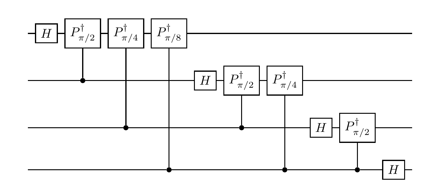
The way that we wrote the QFT in Figure 10.5 is not the conventional way in which it normally appears, since we’re assuming that we measure the result at the end.
In general, we might not want to do this, and instead replace the dependence of the corrective phase gates on the classical measurements by controlled qubits, as shown in Figure 10.6.
We sometimes refer to this as the coherent circuit for the inverse quantum Fourier transform.
One other note about conventions is the difference in ordering of bits between the circuit representation above and the unitary operator definition given before: in the circuit, the least significant bit appears in the first register as opposed to the last, with increasing significance of bits as we go up registers (i.e. down the page).
We could of course introduce a lot of \texttt{SWAP} gates to make these conventions agree, but this is typically unnecessary if we instead just keep track of which qubits are which and remember what we want to do with each one next.