Distinguishing non-orthogonal states
We have already mentioned (Section 4.3) that non-orthogonal states cannot be reliably distinguished, and now we can make this statement more precise.
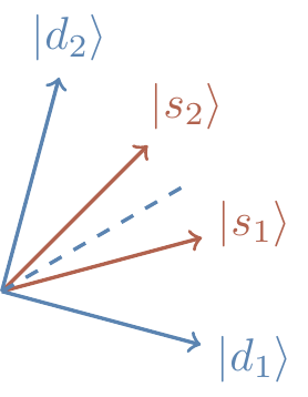
Suppose Alice sends Bob a message by choosing one of the two non-orthogonal states |s_1\rangle and |s_2\rangle, where both are equally likely to be chosen.
What is the probability that Bob will decode the message correctly, and what is the best (i.e. the one that maximises this probability) choice of measurement?
Thinking about what we have already seen, we should expect that how well we can correctly distinguish between |s_1\rangle and |s_2\rangle is directly proportional to “how close” they are to being orthogonal — if they are orthogonal, then we can distinguish perfectly; if they are identical (i.e. collinear), then we cannot distinguish between them at all.
Hopefully, then, our final answer will depend on the angle between |s_1\rangle and |s_2\rangle.
So suppose Bob’s measurement is described by projectors P_1 and P_2, chosen such that “P_1 implies |s_1\rangle, and P_2 implies |s_2\rangle”.
Then
\begin{aligned}
\Pr(\text{success})
&= \frac{1}{2}\left(
\langle s_1|P_1|s_1\rangle + \langle s_2|P_2|s_2\rangle
\right)
\\&= \frac{1}{2}\left(
\operatorname{tr}P_1|s_1\rangle\langle s_1| + \operatorname{tr}P_2|s_2\rangle\langle s_2|
\right)
\\&= \frac{1}{2}\left(
\operatorname{tr}P_1|s_1\rangle\langle s_1| + \operatorname{tr}(\mathbf{1}-P_1)|s_2\rangle\langle s_2|
\right)
\\&= \frac{1}{2}\left(
1 + \operatorname{tr}P_1\left( |s_1\rangle\langle s_1| - |s_2\rangle\langle s_2| \right)
\right).
\end{aligned}
Let us look at the operator D = |s_1\rangle\langle s_1| - |s_2\rangle\langle s_2| that appears in the last expression.
This operator acts on the subspace spanned by |s_1\rangle and |s_2\rangle; it is Hermitian; the sum of its two (real) eigenvalues is zero (whence \operatorname{tr}D=\langle s_1|s_1\rangle-\langle s_2|s_2\rangle=0).
Let us write D as \lambda(|d_+\rangle\langle d_+| - |d_-\rangle\langle d_-|), where |d_\pm\rangle are the two orthonormal eigenstates of D, and \pm\lambda are the corresponding eigenvalues.
Now we write
\begin{aligned}
\Pr (\text{success})
&= \frac{1}{2}\left(
1 + \lambda\operatorname{tr}P_1\left( |d_+\rangle\langle d_+|-|d_-\rangle\langle d_-| \right)
\right)
\\&\leqslant\frac{1}{2}\left(
1+\lambda \langle d_+|P_1|d_+\rangle
\right)
\end{aligned}
where we have dropped the non-negative term \operatorname{tr}P_1|d_-\rangle\langle d_-|.
In fact, it is easy to see that we will maximise the expression above by choosing P_1 = |d_+\rangle\langle d_+| and P_2 = |d_-\rangle\langle d_-|.
The probability of success is then bounded by \frac{1}{2}(1+\lambda).
All we have to do now is to find the positive eigenvalue \lambda for the operator D.
We can do this, of course, by solving the characteristic equation for a matrix representation of D, but, since we are practising using the trace identities, we can also notice that \operatorname{tr}D^2 = 2\lambda^2, and then evaluate the trace of D^2.
We use the trace identities and obtain
\begin{aligned}
\operatorname{tr}D^2
&= \operatorname{tr}\left( |s_1\rangle\langle s_1|-|s_2\rangle\langle s_2| \right) \left( |s_1\rangle\langle s_1|-|s_2\rangle\langle s_2| \right)
\\&= 2-2|\langle s_1|s_2\rangle|^2
\end{aligned}
which gives \lambda = \sqrt{1-|\langle s_1|s_2\rangle|^2}.
Bringing it all together we have the final expression:
\Pr (\text{success})
\leqslant\frac{1}{2}\left( 1+ \sqrt{1-|\langle s_1|s_2\rangle|^2} \right).
We can parametrise |\langle s_1|s_2\rangle| = \cos\alpha, where \alpha is then the angle between |s_1\rangle and |s_2\rangle.
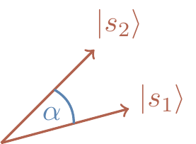
This allows us to express our findings in a clearer way: given two equally likely states, |s_1\rangle and |s_2\rangle, such that |\langle s_1|s_2\rangle| = \cos\alpha, the probability of correctly identifying the state by a projective measurement is bounded by
\Pr (\text{success})
\leqslant\frac{1}{2}(1 + \sin\alpha),
and the optimal measurement that achieves this bound is determined by the eigenvectors of D = |s_1\rangle\langle s_1|-|s_2\rangle\langle s_2| (try to visualise these eigenvectors).
It makes sense, right?
If we try just guessing the state, without any measurement, then we expect \Pr (\text{success}) = \frac{1}{2}.
This is our lower bound, and in any attempt to distinguish the two states we should do better than that.
If the two signal states are very close to each other, then \sin\alpha is small and we are slightly better off than guessing.
As we increase \alpha, the two states become more distinguishable, and, as we can see from the formula, when the two states become orthogonal they also become completely distinguishable.
We will return to this same problem later on, in Section 12.8, where we will use a different, less ad-hoc, approach, working in the more general setting of so-called density operators.