1.7 Quantum decoherence

We do need quantum theory to describe many physical phenomena, but, at the same time, there are many other phenomena where the classical theory of probability works pretty well. Indeed, we hardly see quantum interference on a daily basis. Why? The answer is decoherence. The addition of probability amplitudes, rather than probabilities, applies to physical systems which are completely isolated. However, it is almost impossible to isolate a complex quantum system, such as a quantum computer, from the rest of the world: there will always be spurious interactions with the environment (such as heat transfer), and when we add amplitudes, we have to take into account not only different configurations of the physical system at hand, but also different configurations of the environment.

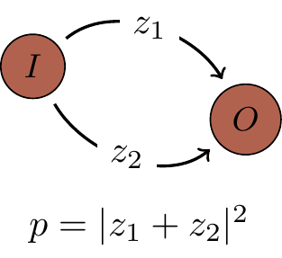
For example, consider an isolated system composed of a quantum computer and its environment. The computer is prepared in some input state I and generates output O. Let us look at the following two scenarios:

1. The computer is isolated and quantum computation does not affect the environment. The computer and the environment evolve independently from each other and, as a result, the environment does not hold any physical record of how the computer reached output O. In this case we add the amplitudes for each of the two alternative computational paths.

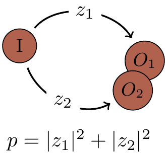
2. Quantum computation affects the environment. The environment now holds a physical record of how the computer reached output O, which results in two final states of the composed system (computer and environment) which we denote O_1 and O_2. We add the probabilities for each of the two alternative computational paths.

When quantum computation affects the environment (or vice versa), we have to include the environment in our analysis, since it is now involved in the computation. Depending on which computational path was taken, the environment may end up in two distinct states. The computer itself may show output O, but when we include the environment we have not one, but two, outputs, O_1 and O_2, denoting, respectively, “computer shows output O and the environment knows that path 1 was taken” and “computer shows output O and the environment knows that path 2 was taken”. There are no alternative ways of reaching O_1 or O_2, hence there is no interference, and the corresponding probabilities read p_1=|z_1|^2 for O_1, and p_2=|z_2|^2 for O_2. The probability that the computer shows output O, regardless the state of the environment, is the sum of of the two probabilities: p=p_1+p_2. We have lost the interference term and, with this, any advantages of quantum computation are also lost. In the presence of decoherence, the interference formula in Equation (\ddagger) is modified and reads p = p_1 + p_2 + 2 v \sqrt{p_1 p_2}\cos (\varphi_2-\varphi_1), where the parameter v, called the visibility of the interference pattern, ranges from 0 (the environment can perfectly distinguish between the two paths, i.e. total decoherence, or no interference) to 1 (the environment cannot distinguish between the two paths, i.e. no decoherence, or full interference), with the values in between corresponding to partial decoherence.

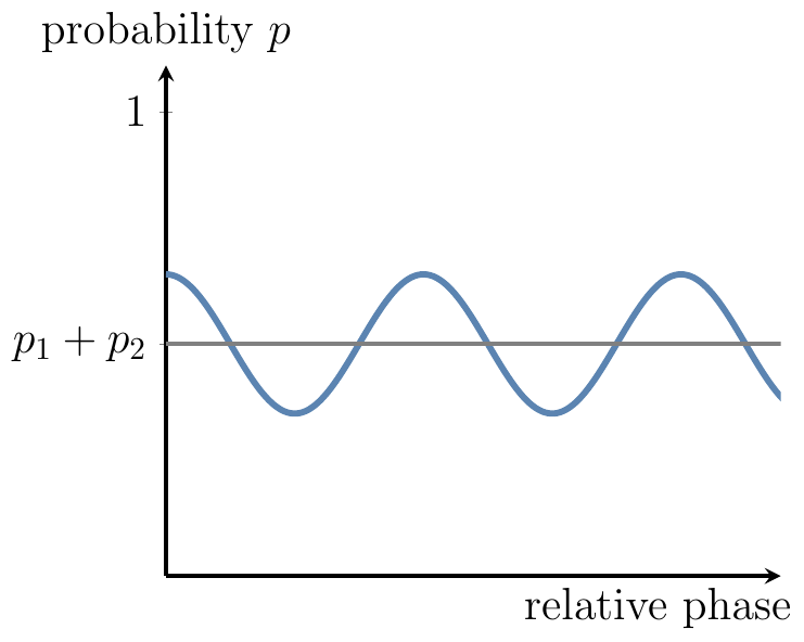
We shall derive this formula later on, and you will see that v quantifies the degree of distinguishability between O_1 and O_2. The more the environment knows about which path was taken, the less interference we see, and the less we can leverage the computational power of quantum effects.

Decoherence suppresses quantum interference.

Decoherence is chiefly responsible for our classical description of the world: without interference terms we may as well add probabilities instead of amplitudes (thus recovering the additivity axiom). While decoherence is a serious impediment to building quantum computers, depriving us of the power of quantum interference, it is not all doom and gloom: there are clever ways around decoherence, such as quantum error correction and fault-tolerant methods, both of which we will meet later.