3.2 Beam-splitters: quantum interference, revisited

One of the simplest quantum devices in which quantum interference can be controlled is a Mach–Zehnder interferometer — see Figure 3.5.⁶⁷

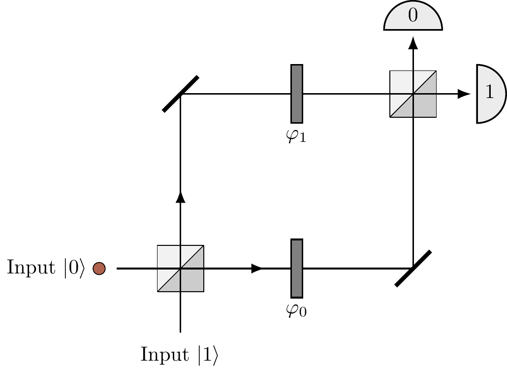
Figure 3.5: The Mach–Zehnder interferometer, with the input photon represented by the coloured dot. This experimental set-up is named after the physicists Ludwig Mach and Ludwig Zehnder, who proposed it back in 1890s.

This is a slightly modified version of the construction shown in Figure 3.2, where we have added two slivers of glass of different thickness into each of the optical paths connecting the two beam-splitters. The slivers are usually referred to as “phase shifters”, and their thicknesses \varphi_0 and \varphi_1 are measured in units of the photon’s wavelength multiplied by 2\pi. These phase shifters are so called because they modify the probability amplitudes by phase factors e^{i\varphi_0} and e^{i\varphi_1}, respectively. The only other change that we make is replacing the symmetric beam-splitters with non-symmetric ones, i.e. they no longer transmit or reflect with equal probability, but instead reflect with some (fixed) probability amplitude i\sqrt{R} and transmit with some probability amplitude \sqrt{T}, where R+T=1. As before, the two input ports of the interferometer are labelled as |0\rangle and |1\rangle, and each of the two output ports, also labelled as 0 and 1, terminates in a photodetector.

A photon (the coloured dot in the figure) impinges on the first beam-splitter from one of the two input ports (here input |0\rangle) and begins its journey towards one of the two photodetectors. Let⁶⁸ U_{ij} denote the probability amplitude that the photon initially in input port j=0,1 ends up in detector i=0,1.

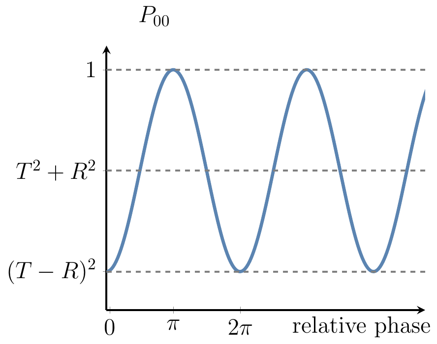
In quantum theory we almost always work with probability amplitudes, and only once we have a full expression for the amplitude of a given outcome do we square its absolute value to get the corresponding probability.

For example, let us calculate U_{00}. We notice that there are two alternative ways for the photon in the input port |0\rangle to end up at the output port 0: It can take the lower path, through the phase shifter \varphi_0, or the upper path, through the phase shifter \varphi_1. The lower path implies two consecutive transmissions at the beam-splitters and the phase factor e^{i\varphi_0}, whereas the upper path implies two consecutive reflections and the phase factor e^{i\varphi_1}. Once the photon ends in the output port 0 there is no way of knowing which path was taken, so we add the amplitudes pertaining to each path. The resulting amplitude is U_{00} = \sqrt{T} e^{i\varphi_0} \sqrt{T} + i\sqrt{R} e^{i\varphi_1} i \sqrt{R}, and the corresponding probability P_{00}=|U_{00}|^2 is \begin{aligned} P_{00} & = \left\vert \sqrt{T}e^{i\varphi_0}\sqrt{T} + i\sqrt{R}e^{i\varphi_1}i\sqrt{R} \right\vert^2 \\&= \left\vert Te^{i\varphi_0} - Re^{i\varphi_1} \right\vert^2 \\& = T^2 + R^2 - 2TR\cos(\varphi_1-\varphi_0). \end{aligned}

The “classical” part of this expression, T^2+R^2, basically says that the photon undergoes either two consecutive transmissions with probability T^2, or two consecutive reflections with probability R^2. The probability of being transmitted through any phase shifter is always 1, hence the phase shifters play no role in the classical description of this process. But the classical description is not correct — it doesn’t agree with physical experiments! — whence the interference term 2TR\cos(\varphi_1-\varphi_0) in which the phase shifters play the essential role. Depending on the relative phase \varphi=\varphi_1-\varphi_0 the probability that the detector 0 “clicks” after having fired a photon into input |0\rangle can vary from (T-R)^2 to 1.

If we do not care about the experimental details, we can represent the action of the Mach–Zehnder interferometer in terms of a diagram, as in Figure 3.6.

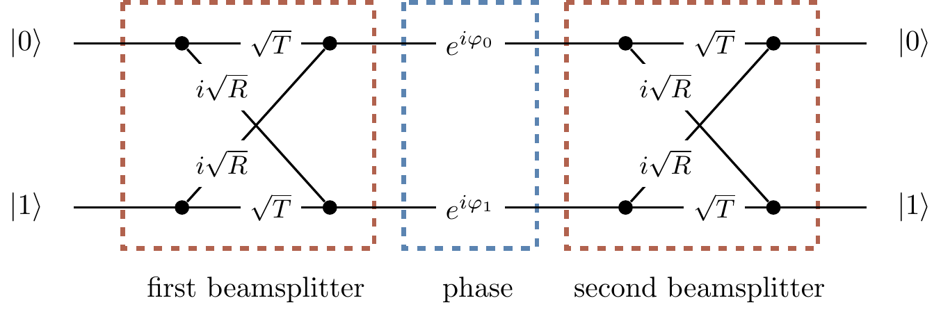
Figure 3.6: The Mach–Zehnder interferometer represented as an abstract diagram.

Here we can follow, from left to right, the multiple different paths that a photon can take in between specific input and output ports. The amplitude along any given path is just the product of the amplitudes pertaining to the path segments (Rule 1, Section 1.1), while the overall amplitude is the sum of the amplitudes for the many different paths (Rule 2, Section 1.1). You can, for example, see that the probability amplitude U_{10} is given by U_{10} = \sqrt{T}e^{i\varphi_0}i\sqrt{R} + i\sqrt{R}e^{i\varphi_1}\sqrt{T} and the corresponding probability is \begin{aligned} P_{10} & = \left\vert \sqrt{T}e^{i\varphi_0}i\sqrt{R} + i\sqrt{R}e^{i\varphi_1}\sqrt{T} \right\vert^2 \\& = 2RT + 2RT\cos(\varphi_1-\varphi_0). \end{aligned} Again, the first term is of “classical” origin and represents probabilities corresponding to each path: one reflection followed by one transmission plus one transmission followed by one reflection, that is, RT+TR=2RT. The second term is the interference term. Clearly, the photon entering port |0\rangle will end up in one of the two detectors, hence P_{00} + P_{10} = R^2 + 2RT + T^2 = (T+R)^2 = 1. The action of the interferometer is thus fully described⁶⁹ by the four probability amplitudes U_{ij} (i,j=0,1).

The most popular instance of a Mach–Zehnder interferometer involves only symmetric beam-splitters (i.e. R=T=\frac{1}{2}) and is fully described by the matrix⁷⁰ U = \begin{bmatrix} -\sin\varphi/2 & \cos\varphi/2 \\\cos\varphi/2 & \sin\varphi/2 \end{bmatrix} where \varphi=\varphi_1-\varphi_0.

---

67. You can play around with a virtual Mach–Zehnder interferometer at Quantum Flytrap’s Virtual Lab. (There are also lots of other things you can do in this virtual lab — go have a look!).↩︎

68. We will often use i as an index even though it is also used for the imaginary unit. Hopefully, no confusion will arise for it should be clear from the context which one is which.↩︎

69. Any isolated quantum device can fully be described by the matrix of probability amplitudes U_{ij} that input j generates output i.↩︎

70. Really, when you write down the matrices describing the action of the symmetric beam-splitters and the phase gates, and then multiply them all together (which is an exercise worth doing!), you actually obtain ie^{i\frac{\varphi_0+\varphi_1}{2}}U rather than U, but as we have already said, we can ignore global phase factors.↩︎