Unitaries as rotations
Now we can finish off our previous discussion (Section 2.10) of the Bloch sphere: we know how single-qubit state vectors correspond to points on the Bloch sphere, but now we can study how (2\times 2) unitary matrices correspond to rotations of this sphere.
Geometrically speaking, the group of (2\times2) unitaries \mathrm{U}(2) is a three-dimensional sphere S^3 in \mathbb{R}^4.
We often make the additional assumption that the determinant is equal to +1, and can then express these matrices as
U = u_0\mathbf{1}+ i(u_x\sigma_x + u_y\sigma_y + u_z\sigma_z).
Such matrices form a very important subgroup of \mathrm{U}(2), called the special (meaning the determinant is equal to 1) unitary group, and denoted by \mathrm{SU}(2).
In quantum theory, any two unitary matrices that differ by some global multiplicative phase factor represent the same physical operation, so we are “allowed to” fix the determinant to be +1, and thus restrict ourselves to considering matrices in \mathrm{SU}(2).
This is a sensible approach, practised by many theoretical physicists, but again, for some historical reasons, this convention is not usually followed in quantum information science.
For example, phase gates are usually written as
P_\alpha = \begin{bmatrix}1&0\\0&e^{i\alpha}\end{bmatrix}
rather than
P_\alpha = \begin{bmatrix}e^{-i\frac{\alpha}{2}}&0\\0&e^{\,i\frac{\alpha}{2}}\end{bmatrix}
Still, as we’ve already mentioned, sometimes the T gate
T
= \begin{bmatrix}1&0\\0&e^{i\pi/4}\end{bmatrix}
= \begin{bmatrix}e^{-i\pi/8}&0\\0&e^{i\pi/8}\end{bmatrix}
is called the \pi/8 gate, because of its \mathrm{SU}(2) form.
Here we’re going to work with \mathrm{SU}(2), so that we can write any (2\times 2) unitary (i.e. up to an overall phase factor) as
U
= u_0\mathbf{1}+ i(u_x \sigma_x + u_y \sigma_y + u_z \sigma_z)
= u_0\mathbf{1}+ i{\vec{u}}\cdot{\vec{\sigma}}
where u_0^2+|\vec{u}|^2=1.
This last restriction on u_0 and \vec{u} allows us to parametrise u_0 and \vec{u} in terms of a real unit vector \vec{n}, parallel to \vec{u}, and a real angle \theta, in such a way that
U
= (\cos\theta)\mathbf{1}+ (i\sin\theta){\vec{n}}\cdot{\vec{\sigma}}.
An alternative way of writing this expression is
U
= e^{i\theta {\vec{n}}\cdot{\vec{\sigma}}},
as follows from the power-series expansion of the exponential.
Indeed, any unitary matrix can always be written in the exponential form as
\begin{aligned}
e^{iA}
&= \mathbf{1}+ iA + \frac{(i A)^2}{1\cdot 2} + \frac{(i A)^3}{1\cdot 2\cdot 3} \ldots
\\&= \sum_{n=0}^\infty \frac{(i A)^n}{n!}
\end{aligned}
where A is an anti-Hermitian matrix.
This is analogous to writing complex numbers of unit modulus as e^{i\alpha}.
Now comes a remarkable connection between two-dimensional unitary matrices and ordinary three-dimensional rotations:
The unitary U = e^{i\theta \vec{n}\cdot\vec{\sigma}} represents a clockwise rotation through the angle 2\theta about the axis defined by \vec{n}.
The fact that the angle is 2\theta, not \theta, comes from our choice of parametrisation; the “better” convention is to parametrise so that U=e^{i\frac{-\theta}{2}\vec{n}\cdot\vec{\sigma}}, and then the direction follows from the right-hand rule, and the rotation corresponds to that in the Bloch sphere.
For example,
\begin{aligned}
e^{i\theta\sigma_x}
&=
\begin{bmatrix}
\cos\theta & i\sin\theta
\\i\sin\theta & \cos\theta
\end{bmatrix}
\\e^{i\theta\sigma_y}
&=
\begin{bmatrix}
\cos\theta & \sin\theta
\\-\sin\theta & \cos\theta
\end{bmatrix}
\\e^{i\theta\sigma_z}
&= \begin{bmatrix}e^{i\theta}&0\\0&e^{-i\theta}\end{bmatrix}
\end{aligned}
represent rotations by 2\theta about the x-, y- and z-axis, respectively.
In fact, these rotations are so important that they get a name.
Rotating a state about a Pauli axis (the x-, y-, or z-axes) is known as a Pauli rotation.
We can write these as
e^{i\theta\sigma_k}
= (\cos\theta)\mathbf{1}+ (i\sin\theta)\sigma_k
for k\in{x,y,z}.
Now we can show that the Hadamard gate
\begin{aligned}
H
&= \frac{1}{\sqrt{2}}
\begin{bmatrix}
1& 1
\\1 & -1
\end{bmatrix}
\\&= \frac{1}{\sqrt{2}}(\sigma_x + \sigma_z)
\\&= (-i)e^{i \frac{\pi}{2} \frac{1}{\sqrt{2}}(\sigma_x+\sigma_z)}
\end{aligned}
represents (since we can ignore the global phase factor of -i) rotation about the diagonal (x+z)-axis by an angle of \pi.
In somewhat abstract terms, we make the connection between unitaries and rotations by looking how the unitary group \mathrm{U}(2) acts on the three-dimensional vector space V of (2\times 2) Hermitian matrices with zero trace.
All such matrices S\in V can be written as S=\vec{s}\cdot\vec{\sigma} for some real \vec{s}, i.e. each matrix is represented by a Euclidean vector \vec{s} in \mathbb{R}^3.
The vector space of traceless matrices (i.e. matrices S such that \operatorname{tr}S=0) might seem like an odd one, but it’s actually one of the fundamental examples of a structure which is fundamental to modern mathematical physics, namely that of a Lie algebra.
These arise when studying Lie groups — which are a combination of groups and manifolds, i.e. “a geometric space which has an algebraic structure” — via the notion of a tangent space.
In particular, the space of (n\times n) traceless skew-Hermitian (A^\dagger=-A) matrices is the Lie algebra known as \mathfrak{su}(2), which is the Lie algebra of \mathrm{SU}(2), since the latter is indeed a Lie group.
You might be wondering why we have suddenly switched to skew-Hermitian instead of Hermitian, but this is really just a mathematician/physicist convention: you can go from one to the other by simply multiplying by i.
For example, mathematicians would usually prefer to work with i\sigma_x, i\sigma_y, and i\sigma_z instead of the Pauli matrices \sigma_x, \sigma_y, and \sigma_z themselves; the former are skew-Hermitian, the latter are Hermitian.
Now, U\in\mathrm{U}(2) acts on the space V by S\mapsto S' = USU^\dagger, i.e.
\vec{s}\cdot\vec{\sigma}
\longmapsto
\vec{s'}\cdot\vec{\sigma}
= U(\vec{s}\cdot\vec{\sigma})U^\dagger
\tag{$\ddagger$}
This gives a linear map \mathbb{R}^3\to\mathbb{R}^3, and is thus given by some (3\times 3) real-valued matrix:
R_U\colon \mathbb{R}^3\to\mathbb{R}^3.
Next, note that this map is an isometry (a distance preserving operation), since it preserves the scalar product in the Euclidean space: for any two vectors \vec{s} and \vec{t},
\begin{aligned}
\vec{s'}\cdot\vec{t'}
&= \frac{1}{2}\operatorname{tr}[S'T']
\\&= \frac{1}{2}\operatorname{tr}[(USU^\dagger)(UTU^\dagger)]
\\&= \frac{1}{2}\operatorname{tr}[ST]
\\&= \vec{s}\cdot\vec{t}
\end{aligned}
(where S=\vec{s}\cdot\vec{\sigma} and T=\vec{t}\cdot\vec{\sigma}) using the cyclic property of the trace.
This means that the matrix R_U is orthogonal: orthogonal transformations preserve the length of vectors as well as the angles between them.
Furthermore, we can show that \det R_U=1.
But the only isometries in three dimensional Euclidean space (which are described by orthogonal matrices with determinant 1) are rotations.
Thus, in the mathematical lingo, we have established a group homomorphism
\begin{aligned}
\mathrm{U}(2) &\longrightarrow \mathrm{SO}(3)
\\U &\longmapsto R_U
\end{aligned}
where \mathrm{SO}(3) stands for the special orthogonal group in three dimensions — the group of all rotations about the origin of three-dimensional Euclidean space \mathbb{R}^3 under the operation of composition, which can be represented by the group of (3\times3) orthogonal (and thus real) matrices.
It follows from Equation (\ddagger) that unitary matrices differing only by a global multiplicative phase factor (e.g. U and e^{i\varphi}U) represent the same rotation.
This mathematical argument is secretly using the language of unit quaternions, also known as versors, since these provide a very convenient way of describing spatial rotation, and are often used in e.g. 3D computer graphics software.
Physicists, however, usually prefer a more direct demonstration of this rotation interpretation, which might go roughly as follows.
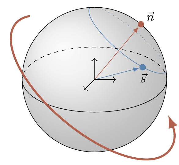
Consider the map \vec{s} \mapsto \vec{s'} induced by U=e^{i \alpha \vec{n}\cdot\vec{\sigma}}.
For small values of \alpha, we can write
\begin{aligned}
\vec{s'}\cdot\vec{\sigma}
&= U(\vec{s}\cdot\vec{\sigma}) U^\dagger
\\&= \Big(
\mathbf{1}+i\alpha (\vec{n}\cdot\vec{\sigma})+\ldots
\Big)
(\vec{s}\cdot\vec{\sigma})
\Big(
\mathbf{1}- i\alpha(\vec{n}\cdot\vec{\sigma})+\ldots
\Big).
\end{aligned}
To the first order in \alpha, this gives
\vec{s'} \cdot\vec{\sigma}
= \Big(
\vec{s} + 2\alpha (\vec{n}\times\vec{s})
\Big)
\cdot \vec{\sigma}
that is,
\vec{s'} =
\vec{s} + 2\alpha(\vec{n}\times\vec{s})
which we recognise as a good old textbook formula for an infinitesimal clockwise rotation of \vec{s} about the axis \vec{n} through the angle 2\alpha.