Types of computation
One single qubit has two logical (i.e. non-superposition) states: |0\rangle and |1\rangle.
Bring another qubit and the combined systems has four logical states: |00\rangle, |01\rangle,|10\rangle, and |11\rangle.
In general n qubits will give us 2^n states, representing all possible binary strings of length n.
It is important to use subsystems — here qubits — rather than one chunk of matter, since, by operating on at most n qubits, we can reach any of the 2^n states of the composed system.
Now, if we let the qubits interact in a controllable fashion, then we are computing!
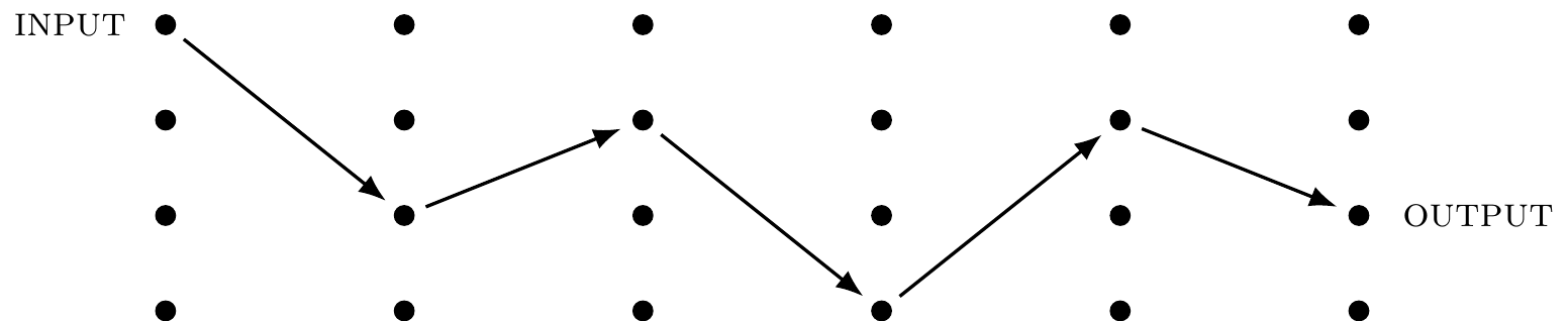
Think about computation as a physical process that evolves a prescribed initial configuration of a computing machine, called \texttt{INPUT}, into some final configuration, called \texttt{OUTPUT}.
We shall refer to the configurations as states.
Figure 1.4 shows five consecutive computational steps performed on four distinct states.
That computation was deterministic: every time you run it with the same input, you get the same output.
But a computation does not have to be deterministic — we can augment a computing machine by allowing it to “toss an unbiased coin” and to choose its steps randomly.
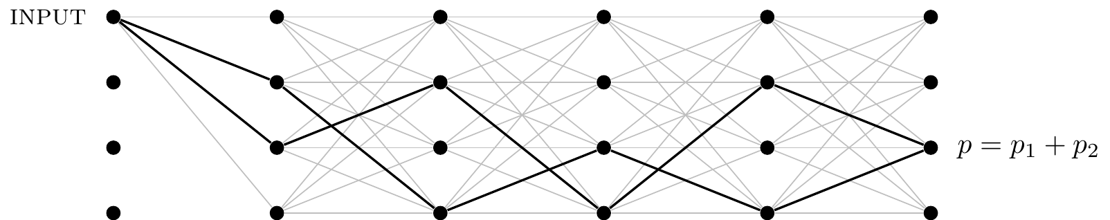
It can then be viewed as a directed tree-like graph where each node corresponds to a state of the machine, and each edge represents one step of the computation, as shown in Figure 1.5
The computation starts from some initial state (\texttt{INPUT}) and it subsequently branches into other nodes representing states reachable with non-zero probability from the initial state.
The probability of a particular final state (\texttt{OUTPUT}) being reached is equal to the sum of the probabilities along all mutually exclusive paths which connect the initial state with that particular state.
Figure 1.5 shows only two computational paths, but, in general, there could be many more paths (here, up to 256) contributing to the final probability.
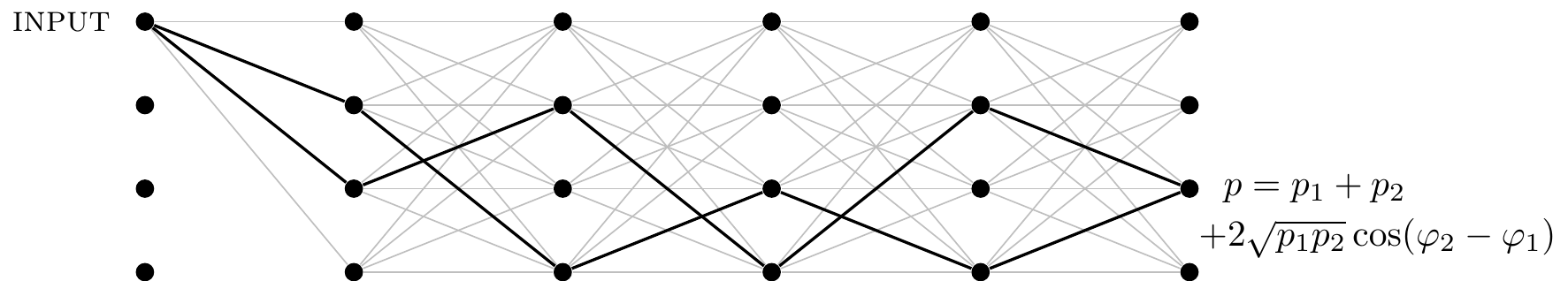
Quantum computation can be represented by a similar graph, as in Figure 1.6.
For quantum computations, we associate with each edge in the graph the probability amplitude that the computation follows that edge.
The probability amplitude that a particular path to be followed is the product of amplitudes pertaining to the transitions in each step.
The probability amplitude of a particular final state being reached is equal to the sum of the amplitudes along all mutually exclusive paths which connect the initial state with that particular state:
z = \sum_{\mathrm{all\,paths}\,k} z_k.
The resulting probability, as we have just seen, is the sum of the probabilities p_k pertaining to each computational path modified by the interference terms.
To show this, note first that
\begin{aligned}
p
&= |z|^2 = z^\star z
\\&= \left( \sum_{j=1}^N z_j \right)^\star
\left( \sum_{k=1}^N z_k \right)
\\&= \left( z_1^\star + z_2^\star + \dots + z_N^\star \right)
\left( z_1 + z_2 + \dots + z_N \right)
\end{aligned}
Multiplying out these two sums gives us terms of the form z_i^\star z_j for 1\leqslant i,j\leqslant N, so we can think of these as forming a square matrix and then split the sum into the “diagonal” terms and the “off-diagonal” terms:
\begin{aligned}
p
&= \underbrace{\sum_k |z_k|^2}_{\substack{\text{diagonal}\\ \text{elements}}}
+ \underbrace{\sum_{\substack{ k > j}} \left( z_k^\star z_j + z_j^\star z_k\right)}_{\substack{\text{off-diagonal}\\ \text{elements}}}
\\&= \sum_k |z_k|^2 + \sum_{\substack{ k > j}} \left( |z_k||z_j|
e^{i(\varphi_j-\varphi_k)}
+ |z_j||z_k|
e^{i(\varphi_k-\varphi_j)}
\right)
\\&= \sum_k |z_k|^2 + \sum_{\substack{ k > j}} \left( |z_k||z_j|
e^{-i(\varphi_k-\varphi_j)}
+ |z_j||z_k|
e^{i(\varphi_k-\varphi_j)}
\right)
\\&= \sum_k p_k + \sum_{k > j} 2 |z_k||z_j|\cos(\varphi_k-\varphi_j)
\\&= \sum_k p_k + \sum_{k > j} \underbrace{2 \sqrt{p_k p_j}\cos(\varphi_k-\varphi_j)}_{\text{interference terms}}.
\end{aligned}
Quantum computation can be viewed as a complex multi-particle quantum interference involving many computational paths through a computing device.
The art of quantum computation is to shape the quantum interference through a sequence of computational steps, enhancing probabilities of the “correct” outputs and suppressing probabilities of the “wrong” ones.