Clifford walks on stabiliser states
There are essentially two ways to define stabiliser states of n qubits.
We have already seen how we can describe them as simultaneous +1 eigenstates of n generators of some stabiliser group \mathcal{S}\leqslant\mathcal{P}_n, but it turns out that we could also define them as the states that are reachable from the |0\rangle^{\otimes n} state using only the \texttt{c-NOT} gate, the Hadamard H, and the phase gate S=\left(\begin{smallmatrix}1&0\\0&i\end{smallmatrix}\right).
If you start playing around with these three gates, you’ll soon notice that you tend to reach certain discrete states, and never anything in between them.
For example, in the single qubit case (so with just the H and S gates), you’ll be able to go between |0\rangle, |1\rangle, |\pm\rangle, and |\pm i\rangle, but never anything like, say, \sqrt{\frac{1}{3}}|0\rangle+\sqrt{\frac{2}{3}}|1\rangle.
When you have two or more qubits, you might also notice that whenever you create an n-qubit superposition that assigns non-zero amplitudes to strings in some set A\subset\{0,1\}^n, it’s always an equal superposition over A (though possibly with \pm1 or \pm i phases), and |A| is always some power of 2.
For example, you can generate states such as \frac{1}{\sqrt{2}}(|000\rangle+|111\rangle)|010\rangle or \frac{1}{2}(|000\rangle+i|100\rangle+|011\rangle-i|111\rangle)|010\rangle, but never states such as \frac{1}{\sqrt{3}}(|001\rangle+|010\rangle+|100\rangle)|010\rangle.
Circuits composed of only \texttt{c-NOT}, H, and S=P_{\pi/2} are special: they effect unitaries that map stabiliser states to stabiliser states.
The n-qubit Clifford group \mathcal{C}_n is the group generated by these three unitaries, and it happens to be exactly the normaliser of of the n-qubit Pauli group inside the group of all (2^n\times2^n) unitary matrices:
\mathcal{C}_n = \{U\in\mathrm{U}(2^n) \mid UPU^\dagger\in\mathcal{P}_n\text{ for all }P\in\mathcal{P}_n\} \eqqcolon N_{\mathrm{U}(2^n)}(\mathcal{P}_n).
It’s a confusing (but immutable) matter of terminology that Clifford gates (i.e. gates made from only unitaries in the Clifford group) are sometimes called stabiliser gates, and Clifford circuits (i.e. circuits made from only Clifford gates) are sometimes called stabiliser circuits, but stabiliser states are never called “Clifford states”.
So if we have an n-qubit stabiliser state, described by n Pauli generators, then any unitary in the Clifford group \mathcal{C}_n will map each of the n Pauli generators to another Pauli generator, and the set of these n new generators will define a new stabiliser state.
Indeed, suppose we have some vector space V stabilised by the group \mathcal{S}, and we apply some unitary operation U.
If |\psi\rangle is an arbitrary element of V, then, for any element S of \mathcal{S},
\begin{aligned}
U|\psi\rangle
&= US|\psi\rangle
\\&= US(U^\dagger U)|\psi\rangle
\\&= (USU^\dagger)U|\psi\rangle
\end{aligned}
and so the state U|\psi\rangle is stabilised by USU^\dagger, from which we deduce that the vector space
UV \coloneqq \{U|\psi\rangle \mid |\psi\rangle\in V\}
is stabilised by the group
U\mathcal{S}U^\dagger \coloneqq \{USU^\dagger \mid S\in\mathcal{S}\}.
Furthermore, if G_1,\ldots,G_r generate \mathcal{S}, then UG_1U^\dagger,\ldots,UG_rU^\dagger generate U\mathcal{S}U^\dagger, so to compute the change in the stabiliser we need only compute how it affects the generators of the stabiliser.
Since the Clifford group is generated by only three elements, we can easily work out how each of these gates acts by conjugation on the Pauli group.
For instance, we have previously seen that the Hadamard gate performs the following transformation:
\begin{aligned}
X
&\longmapsto HXH = Z
\\Z
&\longmapsto HZH = X.
\end{aligned}
Given that Y=iXZ, there is no need to specify the action of H on Y, since we can calculate that
\begin{aligned}
Y\longmapsto
&\,\,i(HXH)(HZH)
\\=&\,\,iZX
\\=&\,\,-Y.
\end{aligned}
All the basic rules for updating stabilisers with Clifford gates can be conveniently tabulated:
| H |
\left\{\begin{matrix}X\longmapsto Z\\Y\longmapsto-Y\\Z\longmapsto X\end{matrix}\right\} |
| S |
\left\{\begin{matrix}X\longmapsto Y\\Y\longmapsto -X\\Z\longmapsto Z\end{matrix}\right\} |
| \texttt{c-NOT} |
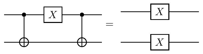
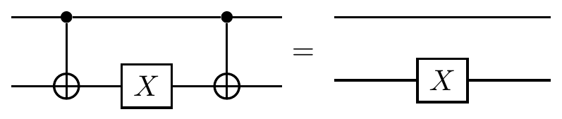
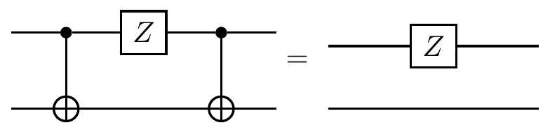
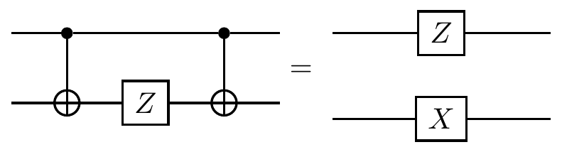
\left\{\begin{matrix}\mathbf{1}X\longmapsto\mathbf{1}X\\X\mathbf{1}\longmapsto XX\\\mathbf{1}Y\longmapsto ZY\\Y\mathbf{1}\longmapsto YX\\\mathbf{1}Z\longmapsto ZZ\\Z\mathbf{1}\longmapsto Z\mathbf{1}\end{matrix}\right\} |
and these rules can be expressed as circuit identities, such as
Let’s work through an example to see how these rules work in practice.
Here’s a simple stabiliser circuit:
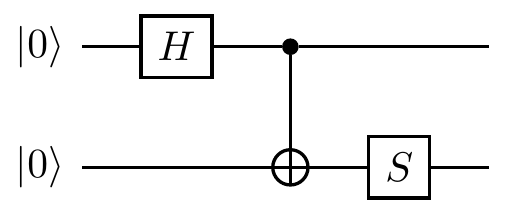
As we step through this circuit we embark on our Clifford walk between two-qubit stabiliser states:
\begin{aligned}
|00\rangle
\overset{H\otimes\mathbf{1}}{\longmapsto}
&\frac{1}{\sqrt{2}}(|0\rangle+|1\rangle)|0\rangle
\\\overset{\texttt{c-NOT}}{\longmapsto}
&\frac{1}{\sqrt{2}}(|00\rangle+|11\rangle)
\\\overset{\mathbf{1}\otimes S}{\longmapsto}
&\frac{1}{\sqrt{2}}(|00\rangle+i|11\rangle).
\end{aligned}
This walk could also be described in terms of stabiliser generators:
\begin{vmatrix}
Z&\mathbf{1}
\\\mathbf{1}&Z
\end{vmatrix}
\overset{H\otimes\mathbf{1}}{\longmapsto}
\begin{vmatrix}
X&\mathbf{1}
\\\mathbf{1}&Z
\end{vmatrix}
\overset{\texttt{c-NOT}}{\longmapsto}
\begin{vmatrix}
X&X
\\Z&Z
\end{vmatrix}
\overset{\mathbf{1}\otimes S}{\longmapsto}
\begin{vmatrix}
X&Y
\\Z&Z
\end{vmatrix}.
Here the first column corresponds to the first qubit, and the second column to the second qubit.
So the first Hadamard gate flips Z\mathbf{1} to X\mathbf{1}, then the \texttt{c-NOT} (which acts on both qubits together, and so acts on entire rows) turns X\mathbf{1} into XX and \mathbf{1}Z into ZZ, then finally the S gate on the second qubit (thus the second column) turns XZ into YZ.
Despite the fact that the Clifford circuits can generate huge entangled n-qubit superpositions starting from the single state |0\rangle^{\otimes n}, such circuits are easy to simulate classically because we can efficiently update the list of stabilisers following the simple rules.
Daniel Gottesman and Emanuel Knill showed that there is a polynomial-time classical algorithm to simulate any stabiliser circuit that acts on a stabiliser state.
We can also efficiently compute the expectation values of any physical observables by examining the updated list of stabilisers.
Note that computing a list of amplitudes would not be efficient, since there are exponentially many of them.
Because they can be efficiently classically simulated, stabiliser circuits necessarily do not capture the full power of quantum computation.
Fully universal quantum computation requires as least one non-Clifford gate, such as the T=\left(\begin{smallmatrix}1&0\\0&e^{-i\pi/4}\end{smallmatrix}\right) gate.
Once we include this gate, we can create circuits that will take us from any initial state, such as |0\rangle^{\otimes n}, to arbitrarily close to any other state in the n-qubit Hilbert space.
Despite this limitation of stabiliser computation, however, it has become a central part of quantum computing, mostly because of its role in quantum error correction and fault-tolerant computation.
Almost all of the quantum error correcting codes are stabiliser codes, and are presented using the stabiliser formalism.