Logical operators …
Here we are going to use the abstract group theory that we developed back in Sections 7.5 and 7.6, but there are other ways of explaining this material.
In Section @(logical-operators-differently) we tell the same story from a different point of view, so if you find this section confusing then don’t worry — you can always come back to it after reading the other one!
It’s always a good idea to have multiple viewpoints.
We have been slowly building up towards constructing quantum error-correction codes using the stabiliser formalism, but there is one major detail that we have yet to mention.
You will perhaps have noticed that we haven’t written out what the stabiliser states actually are, nor what the encoding circuits look like.
There is a simple reason for this: at this point, we don’t actually know!
There’s a little more work to be done — the stabilisers have provided us with a two-dimensional space, but if we have |0\rangle and |1\rangle to encode, how are they mapped within the space?
So far, it’s undefined, and there is a lot of freedom to choose, but the structures provided by group theory are quite helpful here in providing some natural choices.
Furthermore, better understanding these structures is the first step towards figuring out how to upgrade from simple error correction to fault-tolerant computation.
We’re going to turn back all the way to Sections 7.5 and 7.6, where we discovered how to think about normalisers of stabiliser groups inside the Pauli group.
Let’s start with a brief recap.
The n-qubit Pauli group \mathcal{P}_n consists of all n-fold tensor products of Pauli matrices \mathbf{1}, X, Y, and Z, with possible global phase factors \pm1 and \pm i.
Given an operator s\in\mathcal{P}_n, we say that it stabilises a (non-zero) n-qubit state |\psi\rangle if s|\psi\rangle=|\psi\rangle, i.e. if it admits |\psi\rangle as an eigenstate with eigenvalue +1.
We showed that the set of all operators that stabilise every state in a given subspace V form a group, called the stabiliser group; using a little bit of group theory, we characterised all possible stabiliser groups by showing that they are exactly the abelian subgroups of \mathcal{P}_n that do not contain -\mathbf{1}.
Then we looked at the group structure of the Pauli group, and how any stabiliser group \mathcal{S} sits inside it.
It turned out that the normaliser
N(\mathcal{S})
= \{g\in\mathcal{P}_n \mid gsg^{-1}\in\mathcal{S}\text{ for all }s\in\mathcal{S}\}
of \mathcal{S} in \mathcal{P}_n, and the centraliser
Z(\mathcal{S})
= \{g\in\mathcal{P}_n \mid gsg^{-1}=s\text{ for all }s\in\mathcal{S}\}
of \mathcal{S} in \mathcal{P}_n actually agree, because of some elementary properties of the Pauli group.
Furthermore, we showed that the normaliser (or centraliser) was itself normal inside the Pauli group, giving us a chain of normal subgroups
\mathcal{S}
\triangleleft N(\mathcal{S})
\triangleleft \mathcal{P}_n.
This lets us arrange the elements of \mathcal{P}_n into cosets by using the two quotient groups
N(\mathcal{S})/\mathcal{S}
\qquad\text{and}\qquad
\mathcal{P}_n/N(\mathcal{S}).
How does this help us with our stabiliser error-correction codes?
Let’s look first at the former: cosets of \mathcal{S} inside its normaliser N(\mathcal{S}).
If |\psi\rangle\in V_\mathcal{S} is a state in the stabilised subspace, then any element g\in\mathcal{S} always satisfies
g|\psi\rangle
= |\psi\rangle
whereas any element g\in N(\mathcal{S})\setminus\mathcal{S} merely satisfies
g|\psi\rangle
\in V_\mathcal{S}
and, for any such g, there are always states in V_\mathcal{S} that are not mapped to themselves.
However, if we look at cosets of \mathcal{S} inside N(\mathcal{S}) then we discover an incredibly useful fact: all elements of a given coset act on |\psi\rangle in the same way.
To see this, take two representatives for a coset, say g\mathcal{S}=g'\mathcal{S} for g,g'\in N(\mathcal{S}).
By the definition of cosets, this means that there exist s,s'\in\mathcal{S} such that gs=g's'.
In particular then,
gs|\psi\rangle
= g's'|\psi\rangle
but since s,s'\in\mathcal{S} and |\psi\rangle\in V_\mathcal{S}, this says that
g|\psi\rangle
= g'|\psi\rangle
as claimed.
Since the cosets of \mathcal{S} inside N(\mathcal{S}) give well defined actions on stabiliser states, preserving the codespace, we can treat them as operators in their own right.
The cosets of \mathcal{S} inside N(\mathcal{S}) are called logical operators, and any representative of a coset is an implementation for that logical operator.
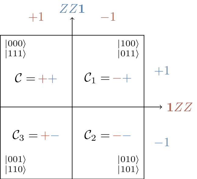
Let’s try to understand this in the context of an example: the three-qubit code from Section 13.1.
The diagram from Section 7.2 was useful in describing this example, so we repeat it as Figure 14.5 below.
To use the terminology of error-correction codes, we are taking our codespace to be
\mathcal{C}
= \langle|000\rangle,|111\rangle\rangle
which is exactly the stabiliser space V_\mathcal{S} of the stabiliser group
\mathcal{S}
= \langle ZZ\mathbf{1},\mathbf{1}ZZ\rangle
and the total eight-dimensional Hilbert space of three qubits is decomposed into four mutually orthogonal two-dimensional subspaces \mathcal{C}\oplus\mathcal{C}_1\oplus\mathcal{C}_2\oplus\mathcal{C}_3 as shown in Figure 14.5.
Since we have chosen a specific basis for each of these subspaces, we should give things a name.
The (orthogonal) basis vectors of the codespace \mathcal{C}=V_\mathcal{S} are called logical states, and are usually taken to be the encodings of |0\rangle and |1\rangle.
In general, the logical states will be superpositions of states, but we still sometimes refer to them as codewords.
In our example of the three-qubit code, we have the two logical states logical 0 and logical 1, which we denote by
\begin{aligned}
|0\rangle_L
&\coloneqq |000\rangle
\\|1\rangle_L
&\coloneqq |111\rangle.
\end{aligned}
The justification for these names is twofold: firstly, |0\rangle_L is exactly the encoding of |0\rangle, the “actual” zero state; and secondly, this state |0\rangle_L will behave exactly as the zero state should when acted upon by the logical operators.
For example, the operator X sends |0\rangle to |1\rangle, so the logical X should send the logical |0\rangle to the logical |1\rangle.
Let’s make this happen!
The normaliser of \mathcal{S} inside \mathcal{P}_3 is
N(\mathcal{S})
= \{\mathbf{1},XXX,-YYY,ZZZ\} \times \mathcal{S}
which we have written in such a way that we can just read off the cosets: there are four of them, and they are represented by \mathbf{1}, XXX, -YYY, and ZZZ.
These four (implementations of) logical operators all get given the obvious names:
\begin{aligned}
\mathbf{1}_L
&\coloneqq \mathbf{1}
\\X_L
&\coloneqq XXX
\\Y_L
&\coloneqq -YYY
\\Z_L
&\coloneqq ZZZ
\end{aligned}
But note that these are not necessarily the smallest weight implementations!
For example, any single Z_i (i.e. a Z acting on the i-th qubit) will have the same logical effect as ZZZ, as we can see by looking at how it acts on the logical states:
\begin{aligned}
Z_1|1\rangle_L
&= Z\mathbf{1}\mathbf{1}|111\rangle
\\&= -|111\rangle
\\&= ZZZ|111\rangle
\\&= ZZZ|1\rangle_L.
\end{aligned}
In contrast, XXX is the smallest weight logical X implementation.
The natural question to ask is then how to find all the implementations, but this is answered by going back to the very definition of them as coset representatives: if P is some implementation of a logical operator, then so too is SP for any S\in\mathcal{S}.
In the example above, we see that Z_1=Z\mathbf{1}\mathbf{1} is exactly \mathbf{1}ZZ\cdot ZZZ.
Because of this, we should really write something like Z_L=ZZZ\mathcal{S}, or Z_L=[ZZZ], to make clear that ZZZ is just one specific representation of Z_L, but you will find that people often conflate implementations with the logical operators themselves and simply write Z_L=ZZZ.
Generally, for any CSS code encoding a single qubit into n-qubits, we define the logical X and logical Z operators to be the (equivalence classes of) the tensor products of all X operators or all Z operators (respectively), i.e.
\begin{aligned}
X_L
&\coloneqq X^{\otimes n}
\\Z_L
&\coloneqq Z^{\otimes n}.
\end{aligned}
Even more generally, for any [[n,k,d]] code constructed from a stabiliser \mathcal{S}, it will be the case that N(\mathcal{S})/S\cong\mathcal{P}_k.
Just a warning before moving on: this discussion might make logical states sound pointlessly simple — logical 0 is just given by three copies of |0\rangle, so what’s the point?
But this apparent simplicity is due to the fact that the three-qubit code is somehow not very quantum at all (these logical states are not superpositions), and in general things get a lot more complicated.
For example, even with the three-qubit code, we shall see in Section ?? that
|+\rangle_L
\neq |{+}{+}{+}\rangle
where, as per usual, |+\rangle=H|0\rangle=(|0\rangle+|1\rangle)/2.