Discretisation of quantum errors
When a quantum computer interacts and becomes entangled with its environment, it impacts the environment in such a way that the environment maintains a physical record of how the computer arrived at the desired output.
Here, in our simplistic diagram, we consider only two computational paths.
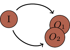
With decoherence present, quantum computation spills out the environment and results in not one, but two output states:
\begin{aligned}
|O_1\rangle
&\coloneqq |O\rangle|e_1\rangle
\\&= \text{``computer shows output $O$, environment knows that path 1 was taken''}
\\|O_2\rangle
&\coloneqq |O\rangle|e_2\rangle
\\&= \text{``computer shows output $O$, environment knows that path 2 was taken''}
\end{aligned}
The two final states O_1 and O_2 are identical if and only if |\langle e_1|e_1\rangle|=1.
In this case, the environment does not know anything about what happened during the computation — there is quantum interference — and we add probability amplitudes corresponding to the two computational paths.
In contrast, the two final states O_1 and O_2 are completely different if and only if |\langle e_1|e_2\rangle|=0.
Then there is only one path to the output — there is no quantum interference — and there is nothing to add.
Of course, there are also midway cases 0<|\langle e_1|e_2\rangle|<1 corresponding to partial distinguishability of the final states.
If we wish to study the evolution of the qubit alone, then we can do so in terms of density operators: it evolves from the pure state |\psi\rangle\langle\psi| to a mixed state, which can be obtained by tracing over the environment.
We know that the state vector |\psi\rangle=\alpha|0\rangle+\beta|1\rangle evolves as
\left( \alpha|0\rangle +\beta |1\rangle\right)|e\rangle \longmapsto
\alpha |0\rangle|e_{00}\rangle +\beta |1\rangle |e_{11}\rangle
and we can write this as the evolution of the projector |\psi\rangle\langle\psi|, and then trace over the environment to obtain
\begin{aligned}
|\psi\rangle\langle\psi| \longmapsto & |\alpha|^2|0\rangle\langle 0| \langle e_{00}|e_{00}\rangle+ \alpha\beta^\star |0\rangle\langle 1|\langle e_{11}|e_{00}\rangle
\\+ &\alpha^\star\beta |1\rangle\langle 0|\langle e_{00}|e_{11}\rangle + |\beta|^2|1\rangle\langle 1|\langle e_{11}|e_{11}\rangle.
\end{aligned}
Written in matrix form, this is
\begin{bmatrix}
|\alpha|^2 & \alpha\beta^\ast
\\\alpha^\ast\beta & |\beta|^2
\end{bmatrix}
\longmapsto
\begin{bmatrix}
|\alpha|^2 & \alpha\beta^\ast \langle e_{11}|e_{00}\rangle
\\\alpha^\ast\beta \langle e_{00}|e_{11}\rangle & |\beta|^2
\end{bmatrix}.
The off-diagonal elements (originally called coherences) vanish as \langle e_{00}|e_{11}\rangle approaches zero.
This is why this particular interaction is called decoherence.
Notice that
|\psi\rangle|e\rangle \longmapsto \mathbf{1}|\psi\rangle|e_{\mathbf{1}}\rangle+Z|\psi\rangle|e_Z\rangle,
implies
|\psi\rangle\langle\psi|\longmapsto \mathbf{1}|\psi\rangle\langle\psi| \mathbf{1}\langle e_{\mathbf{1}}|e_{\mathbf{1}}\rangle +Z|\psi\rangle\langle\psi| Z\langle e_Z|e_Z\rangle,
only if \langle e_{\mathbf{1}}|e_Z\rangle=0, since otherwise we would have additional cross terms \mathbf{1}|\psi\rangle\langle\psi|Z and Z|\psi\rangle\langle\psi|\mathbf{1}.
In this case (i.e. when \langle e_{\mathbf{1}}|e_Z\rangle=0) we can indeed say that, with probability \langle e_{\mathbf{1}}|e_{\mathbf{1}}\rangle, nothing happens, and, with probability \langle e_Z|e_Z\rangle, the qubit undergoes the phase-flip Z.
We can also represent this with the Kraus operators
\begin{aligned}
E_0
&= \sqrt{|e_\mathbf{1}\rangle\langle e_\mathbf{1}|} \mathbf{1}
\\E_1
&= \sqrt{|e_Z\rangle\langle e_Z|} Z
\end{aligned}
which can be shown to satisfy E_0^\dagger E_0+E_1^\dagger E_1=\mathbf{1}.
The process of decoherence is continuous.
It involves the environment gradually acquiring information about computational paths and the associated relative environmental states (|e_0\rangle and |e_1\rangle in our example above), which evolve over time to become increasingly orthogonal to one another.
Despite this, we can perceive the influence of the environment on our system of interest — a collection of qubits in a quantum computer — in terms of discrete operations.
In essence, we can digitise quantum errors.