12.11 Remarks and exercises

12.11.1 Operator decompositions

Analogously to how we can factor polynomials into linear parts, or factor numbers into prime divisors, we can “factor” matrices into smaller components. Doing so often helps us to better understand the geometry of the situation: we might be able to understand the transformation described by a single matrix as “some reflection, followed by some rotation, followed by some scaling”. For us, one specific use of such a “factorisation” (known formally as an operator decomposition) is in better understanding various operator norms, as we explain in Exercise 12.11.2.

Here are three operator decompositions that are particularly useful in quantum information theory. The second is for arbitrary operators between Hilbert spaces, the first and third are for normal endomorphisms (i.e. normal operators from one Hilbert space to itself).

1. Spectral decomposition. Recall Section 4.5: the spectral theorem tells us that every normal operator A\in\mathcal{B}(\mathcal{H}) can be expressed as a linear combination of projections onto pairwise orthogonal subspaces. We write the spectral decomposition of A as A = \sum_k \lambda_k |v_k\rangle\langle v_k| where \lambda_k are the eigenvalues of A, with corresponding eigenvectors |v_k\rangle, which form an orthonormal basis in \mathcal{H}.

In matrix notation, we can write this as A = UDU^\dagger where D is the diagonal matrix whose diagonal entries are the eigenvalues \lambda_k, and where U is the unitary matrix whose columns are the eigenvectors |v_k\rangle.

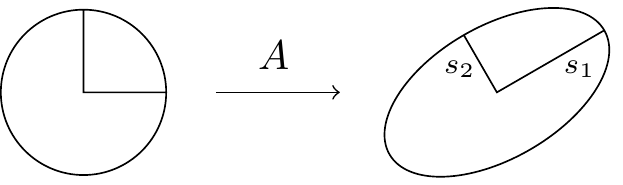
2. Singular value decomposition (SVD). We have already mentioned the SVD in Exercise 5.14.13 when discussing the Schmidt decomposition, but we recall the details here. Consider any (non-zero) operator A\in\mathcal{B}(\mathcal{H},\mathcal{H}'). From this, we can construct two positive semi-definite operators: A^\dagger A\in\mathcal{B}(\mathcal{H}) and AA^\dagger\in\mathcal{B}(\mathcal{H}'). These are both normal, and so we can apply the spectral decomposition to both. In particular, if we denote the eigenvalues of A^\dagger A by \lambda_k, and the corresponding eigenvectors by |v_k\rangle, then we see that the vectors |u_k\rangle \coloneqq \frac{1}{\sqrt{\lambda_k}}A|v_k\rangle form an orthonormal system in \mathcal{H}' (and are, in fact, eigenvectors of AA^\dagger), since \begin{aligned} \langle u_i|u_j\rangle &= \frac{1}{\sqrt{\lambda_i}\sqrt{\lambda_j}} \langle v_i|A^\dagger A|v_j\rangle \\&= \frac{\lambda_j}{\sqrt{\lambda_i}\sqrt{\lambda_j}} \langle v_i|v_j\rangle \\&= \delta_{ij}. \end{aligned} We define the singular values s_k of A to be the square roots of the eigenvalues of A^\dagger A, i.e. s_k^2=\lambda_k. These singular values satisfy A|v_k\rangle=s_k|u_k\rangle by construction, and so we can write A = \sum_k s_k|u_k\rangle\langle v_k| which we call the singular value decomposition (or SVD). This decomposition holds for arbitrary (non-zero) operators as opposed to just normal ones, and also for operators between two different Hilbert spaces as opposed to just endomorphisms. In words, this decomposition says that, given A, we can find orthonormal bases of \mathcal{H} and \mathcal{H}' such that A maps the k-th basis vector of \mathcal{H} to a non-negative multiple of the k-th basis vector of \mathcal{H}' (and sends any left over basis vectors to 0, if \dim\mathcal{H}>\dim\mathcal{H}').

In matrix notation, we can write this as A = U\sqrt{D}V^\dagger where D is the diagonal matrix of eigenvalues (and so \sqrt{D} is the diagonal matrix of singular values), and both U and V are unitary.

Geometrically, we are decomposing any linear transformation into a composition of a rotation or reflection V^\dagger, followed by a scaling by the singular values \sqrt{D}, followed by another rotation or reflection U. This maps the unit sphere in \mathcal{H} onto an ellipsoid in \mathcal{H}', and the singular values of A are exactly the lengths of the semi-axes of this ellipsoid.

3. Polar decomposition. Let A\in\mathcal{B}(\mathcal{H}) be a normal arbitrary operator. Since it is an endomorphism, it is represented by a square matrix. Forgetting that A is normal for a moment, we know that its SVD takes the form \begin{aligned} A &= U\sqrt{A^\dagger A} \\&= \sqrt{AA^\dagger}U \end{aligned} where the unitary matrix U connects the two eigenbases: U=\sum_k|u_k\rangle\langle v_k|. We shall return to this unitary U shortly.

Since A is normal, A^\dagger A=AA^\dagger, so we can define its modulus as |A| \coloneqq \sqrt{A^\dagger A} which gives us the polar decomposition A = |A|U. This is the matrix analogue of the polar decomposition of a complex number: z=re^{i\theta}.

If we decompose the eigenvalues of A as \lambda_k=r_k e^{i\theta_k} (with corresponding eigenvectors |v_k\rangle) then the spectral decomposition of A gives us \begin{aligned} A &= \sum_k \lambda_k|v_k\rangle\langle v_k| \\&= \sum_k r_ke^{i\theta_k}|v_k\rangle\langle v_k| \\&= \sum_k r_k|u_k\rangle\langle v_k| \end{aligned} where |u_k\rangle=e^{i\theta_k}|v_k\rangle, so we see that the unitary U=\sum_k|u_k\rangle\langle v_k| in the polar decomposition contains all the information of the phase factors.

12.11.2 More operator norms

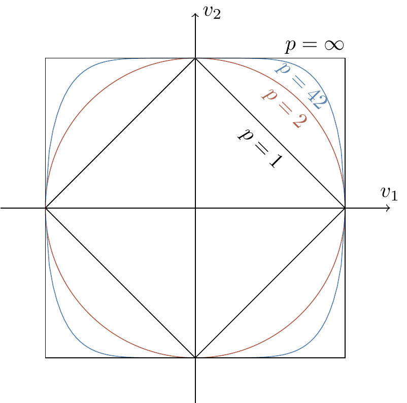
We have already seen, all the way back in Section 1.11.2²⁵³, how the Euclidean norm (from which we get the Euclidean distance) is the special case p=2 of p-norms (also known as \ell^p-norms), where \|v\|_p \coloneqq \left( \sum_{i=1}^n |v_i|^p \right)^{\frac{1}{p}} for a vector v=(v_1,\ldots,v_n)\in\mathbb{R}^n, and for p\in\mathbb{N}. We can actually extend this definition to include the case p=\infty by setting \|v\|_\infty \coloneqq \max_{1\leqslant i\leqslant n}|v_i|. One particularly nice consequence of this definition is that \|v\|_1 \geqslant\|v\|_2 \geqslant\ldots \geqslant\|v\|_\infty for any vector v.

You might recall that we named the Cauchy–Schwartz inequality as arguably the most useful inequality in analysis. Well it turns out that it is actually the special case p=2 of an inequality concerning p-norms.

Hölder’s inequality. Let p,q\in\mathbb{N}\cup\{\infty\} be such that \frac{1}{p}+\frac{1}{q}=1. Then \|vw\|_1 \leqslant\|v\|_p\|w\|_q with equality if and only if v and w are “(p,q)-linearly dependent”.

We will come back to the relevance of these p-norms shortly. For now, let us introduce three norms (two of which we have already seen, but recall here again to tell a more complete story) on the space of endomorphisms \mathcal{B}(\mathcal{H}) of a Hilbert space, each of which can be defined neatly in terms of singular values. Note that, if A is normal, then we its singular values are exactly the absolute values of its eigenvalues, which usually lets us simplify the definition of the norm.

Throughout, let A\in\mathcal{B}(\mathcal{H}), with singular values s_k.

1. Spectral norm. This one is so frequently used that it is often simply called the operator norm and denoted simply by \|\cdot\|. It is the maximum length of the vector A|v\rangle over all possible normalised vectors |v\rangle\in\mathcal{H}, i.e. \|A\| \coloneqq \max_{|v\rangle\in S_{\mathcal{H}}^1}\Big\{ |A|v\rangle| \Big\} (where S_{\mathcal{H}}^1 is the unit sphere in \mathcal{H}, i.e. the set of vectors of norm 1). From this definition, one can actually show that the norm is given by the largest singular value: \|A\| = \max_k s_k.

2. Trace norm. This is given by the sum of the singular values of A, i.e. \|A\|_{\operatorname{tr}} \coloneqq \sum_k s_k but note that we can rewrite this using the polar decomposition (from Section 12.11.1) as simply \|A\|_{\operatorname{tr}} = \operatorname{tr}|A|.

3. Frobenius norm. We have mentioned a few times how inner products give rise to norms, and you might remember that we introduced an inner product on \mathcal{B}(\mathcal{H}) a while ago: the Hilbert–Schmidt norm²⁵⁴ \begin{aligned} (A|B) &\coloneqq \operatorname{tr}A^\dagger B \\&= \sum_{i,j} A_{ij}^\star B_{ji}. \end{aligned} The Frobenius norm is the norm induced by this inner product, i.e. \begin{aligned} \|A\|_F &\coloneqq \sqrt{(A|A)} \\&= \sqrt{\operatorname{tr}(A^\dagger A)} \\&= \sqrt{\sum_{i,j}|A_{ij}|^2}. \end{aligned}

Let’s study the relation between the operator norm and the trace norm first. By definition, we see that \|A\|_{\operatorname{tr}} \geqslant\|A\| but there is another, more subtle, inequality that they satisfy, namely |(A|B)| \leqslant\|A\|_{\operatorname{tr}}\|B\| which is like a more general version of the Cauchy–Schwartz inequality, and is sometimes referred to as Hölder’s inequality for matrices. To derive this inequality, we can use the SVD of A, since then \begin{aligned} |(A|B)| &= |\operatorname{tr}A^\dagger B| \\&= \left| \operatorname{tr}\left( \sum_k s_k|v_k\rangle\langle u_k| B \right) \right| \\&= \left| \sum s_k\langle u_k|B|v_k\rangle \right| \\&\leqslant\sum_k s_k|\langle u_k|B|v_k\rangle| \\&\leqslant\sum_k s_k\|B\| \\&= \|A\|_{\operatorname{tr}}\|B\|. \end{aligned}

We can actually use this inequality to recover either the operator or the trace norm, by maximising: for any fixed A (or any fixed B), we can obtain equality: \begin{aligned} \|A\|_{\operatorname{tr}} &= \max_{\|B\|=1}\{(A|B)\} \\\|B\| &= \max_{\|A\|_{\operatorname{tr}}=1}\{(A|B)\}. \end{aligned} To see this, in the first case we can use the polar decomposition A=|A|U to see that equality is attained by B=U; in the second case we can use the polar decomposition B=|B|V to see that equality is attained by A=V|v_1\rangle\langle v_1|, where |v_1\rangle is the eigenvector of |B| with the largest eigenvalue (or, equivalently, singular value). In particular, this gives us a variational characterisation of the trace norm which is very useful at times: \|A\|_{\operatorname{tr}} = \max_{U\text{ unitary}}|\operatorname{tr}AU|.

One final special case to point out is what happens if A is Hermitian. Then we can separate the spectral decomposition into positive and negative parts, and write A as the difference of two positive operators: A = A_+ - A_-. Then \begin{aligned} |A| &= A_+ + A_- \\\|A\|_{\operatorname{tr}} &= \operatorname{tr}A_+ + \operatorname{tr}A_-. \end{aligned}

Now we finally return to the relevance of p-norms: it turns out that all these three operator norms above are actually special cases of Schatten p-norms. For p\in\mathbb{N} we define the Schatten p-norm in terms of singular values s_k as \|A\|_p \coloneqq \left( \sum_k |s_k|^p \right)^\frac{1}{p} and we define \|A\|_\infty \coloneqq \max_k |s_k| analogously to how we did for \ell^p-norms. We then recover the trace norm, the Frobenius norm, and the spectral norm by taking p=1,2,\infty, respectively: \begin{aligned} \|A\|_1 &= \|A\|_{\operatorname{tr}} \\\|A\|_2 &= \|A\|_F \\\|A\|_\infty &= \|A\|. \end{aligned} All Schatten p-norms are sub-multiplicative (\|AB\|_p\leqslant\|A\|_p\|B\|_p) and unitarily invariant (\|A\|=\|UAV\| for any unitaries U and V).

12.11.3 Fidelity in a trace norm inequality

There is a useful inequality involving the trace norm: \operatorname{tr}(A-B)^2 \leqslant\|A^2-B^2\|_{\operatorname{tr}}. Let’s prove it!

Let \lambda_k be the eigenvalues of the operator A-B, with corresponding eigenvectors and |u_k\rangle. Then \operatorname{tr}(A-B)^2 = \sum_k \lambda_k^2 since the trace is exactly the sum of eigenvalues. Now, for any unitary U, we have that \|A^2-B^2\|_{\operatorname{tr}} \geqslant|\operatorname{tr}(A^2-B^2)U| since \|X\|_{\operatorname{tr}}=\max_{U\text{ unitary}} |\operatorname{tr}(XU)|. If we take U=\sum_i\pm|u_k\rangle\langle u_k|, where the signs are chosen so that each term \langle u_k|A^2-B^2|u_k\rangle is non-negative, then \begin{aligned} \|A^2-B^2\|_{\operatorname{tr}} &\geqslant|\operatorname{tr}(A^2-B^2)U| \\&= \sum_k |\langle u_k|A^2-B^2||u_k\rangle|. \end{aligned}

Writing A^2-B^2 as²⁵⁵ A^2-B^2 = \frac{1}{2}\Big[ (A+B)(A-B) + (A-B)(A+B) \Big] we see that \begin{aligned} \langle u_k|A^2-B^2||u_k\rangle &= \frac{1}{2}\langle u_k|(A+B)(A-B) + (A-B)(A+B)|u_k\rangle \\&= \lambda_i\langle u_k|A+B|u_k\rangle. \end{aligned} Then, since \lambda_i=\langle u_k|A|u_k\rangle-\langle u_k|B|u_k\rangle is the difference of two non-negative numbers, we have that \langle u_k|A+B|u_k\rangle \geqslant|\lambda_i|. Putting this all together, we obtain \begin{aligned} \|A^2-B^2\|_{\operatorname{tr}} &\geqslant\sum_k |\langle u_k|A^2-B^2||u_k\rangle| \\&\geqslant\sum_k \lambda_k^2 \\&= \operatorname{tr}(A-B)^2 \end{aligned} as desired.

One particularly nice application of this inequality arises when we take A=\sqrt{\rho} and B=\sqrt{\sigma}, since then \operatorname{tr}(\sqrt{\rho}-\sqrt{\sigma})^2 \leqslant\|\rho-\sigma\|_{\operatorname{tr}} or, after some rearrangement, 1-\operatorname{tr}(\sqrt{\rho}\sqrt{\sigma}) \leqslant\frac{1}{2}\|\rho-\sigma\|_{\operatorname{tr}} and we recognise \operatorname{tr}(\sqrt{\rho}\sqrt{\sigma}) as the fidelity.

12.11.4 Hamming distance

Show that the Hamming distance (defined in Section 12.1) is indeed a metric.

12.11.5 Operator norm

Prove the following properties of the operator norm:

1. \|A\otimes B\|=\|A\|\|B\| for any operators A and B
2. If A is normal, then \|A^\dagger\|=\|A\|
3. If U is unitary, then \|U\|=1
4. If P\neq0 is an orthogonal projector, then \|P\|=1.

Using the singular value decomposition²⁵⁶, or otherwise, prove that the operator norm has the following two properties for any operators A and B:

5. Unitary invariance: \|UAV\|=\|A\| for any unitaries U and V
6. Sub-multiplicativity: \|AB\|\leqslant\|A\|\|B\|.

Recall that we say that V approximates U with precision \varepsilon if \|U-V\|\leqslant\varepsilon.

7. Prove that, if V approximates U with precision \varepsilon, then V^{-1} approximates U^{-1} with the same precision \varepsilon.

Using the Cauchy–Schwartz inequality, or otherwise, prove the following, for any vector |\psi\rangle and any operators A and B:

8. |\langle\psi|A^\dagger B|\psi\rangle|\leqslant\|A\|\|B\|.

12.11.6 Tolerance and precision

Suppose we wish to implement a quantum circuit consisting of gates U_1,\ldots,U_d, but we only have available to us gates V_1,\ldots,V_d. Luckily, these gates happen to be pretty good approximations to our desired gates, and the error is uniform: \|U_i-V_i\|\leqslant\varepsilon for all i=1,\ldots,d for some fixed \varepsilon.

We want our approximate circuit to be within some tolerance \delta of the desired circuit: the probabilities of different outcomes of V=V_d\cdots V_1 should be be within \delta of the “correct” probabilities of the different outcomes of U=U_d\cdots U_1, i.e. |p_U-p_V|\leqslant\delta.

How small must \varepsilon be with respect to \delta in order for us to achieve this?²⁵⁷

12.11.7 Statistical distance and a special event

1. Show that, if p and q are probability distributions on the same sample space \Omega, then d(p,q) = \max_{A\subseteq\Omega}\{|p(A)-q(A)|\}.
2. By definition, the above maximum is realised for some specific subset A\subseteq\Omega, i.e. there exists some event (described by the set of outcomes A) that is optimal in distinguishing p from q. What is this event?

12.11.8 Joint probability distributions

If we simultaneously sample two random variables from the same probability space, then we obtain a joint distribution: r(x,y) \coloneqq \Pr(x\text{ and }y). From this we can recover the marginals \begin{aligned} p(x) &\coloneqq \sum_y r(x,y) \\q(y) &\coloneqq \sum_x r(x,y). \end{aligned}

So let r(x,y) be a joint probability distribution with marginals p(x) and q(y). Show that²⁵⁸ d_{\operatorname{tr}}(p,q) \leqslant\Pr(x\neq y) \equiv \sum_{\{x,y\mid x\neq y\}} p(x,y).

12.11.9 Distinguishability and the trace distance

Say we have a physical system which is been prepared in one of two states (say, \rho_0 and \rho_1), each with equal probability. Then, as shown in Section 12.8, a single measurement can distinguish between the two preparations with probability at most \frac{1}{2}[1+d_{\operatorname{tr}}(\rho_0,\rho_1)].

1. How does this probability change if the states \rho_0 and \rho_1 are not equally liked, but instead sent with some predetermined probabilities p_0 and p_1, respectively?

2. Suppose that you are given one randomly selected qubit from a pair in the state |\psi\rangle = \frac{1}{\sqrt{2}}\left( |0\rangle\otimes\left( \sqrt{\frac23}|0\rangle - \sqrt{\frac13}|1\rangle \right) + |1\rangle\otimes\left( \sqrt{\frac23}|0\rangle + \sqrt{\frac13}|1\rangle \right) \right) from Exercise 8.8.1. What is the maximal probability with which we can determine which qubit (either the first or the second) we were given?

---

253. Think how far you’ve come since then!↩︎

254. Here we drop the factor of \frac{1}{2} that we sometimes included for simplifying certain calculations.↩︎

255. This is the non-commutative version of the identity a^2-b^2=(a+b)(a-b).↩︎

256. Recall Exercise 5.14.13↩︎

257. Hint: recall that |p_U-p_V|\leqslant 2\|U-V\|.↩︎

258. Hint: \begin{aligned}d_{\operatorname{tr}}(p,q)&= 1 - \sum_x \min\{p(x),q(x)\}\\&\leqslant 1 - \sum_x p(x,x)\\&= \Pr(x\neq y).\end{aligned}↩︎