The three-qubit code
In Section 9.3 we met the notion of isometries: operators V that map one Hilbert space to another and satisfy V^\dagger V=\mathbf{1}.
This implies that isometries can be reversed, or corrected: we can apply V^\dagger and end up exactly how we started.
We say that a quantum channel \mathcal{E}\colon\mathcal{B}(\mathcal{H})\to\mathcal{B}(\mathcal{H}') is correctable if there exists a recovery channel \mathcal{R}\colon\mathcal{B}(\mathcal{H}')\to\mathcal{B}(\mathcal{H}) such that the composition \mathcal{R}\circ\mathcal{E} is the identity channel \mathbf{1}.
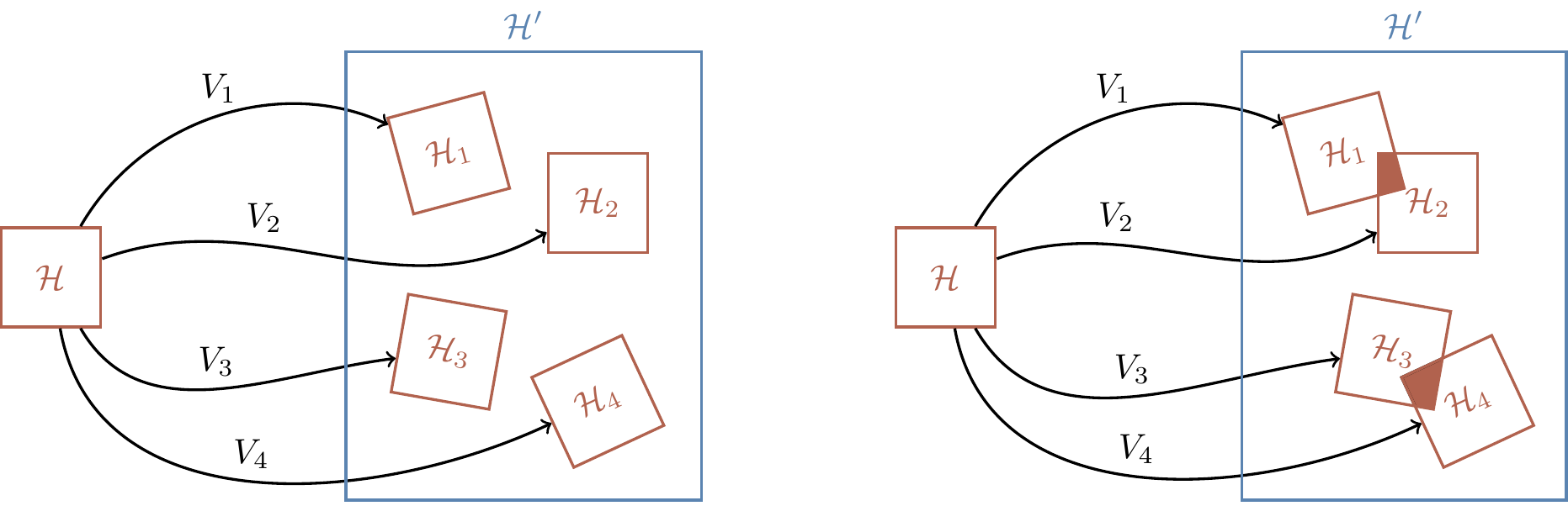
Now suppose we have isometries V_1,\ldots,V_n\colon\mathcal{H}\to\mathcal{H}'.
If \mathcal{H}' is “sufficiently bigger” than \mathcal{H}, and if the images \mathcal{H}'_i\coloneqq V_i(\mathcal{H}) do not overlap then we can reverse the action of the channel given by a statistical mixture of the V_i:
we can, at least in principle, perform a measurement on \mathcal{H}', defined by the partition \mathcal{H}'=\mathcal{H}'_1\oplus\mathcal{H}'_2\oplus\ldots\oplus\mathcal{H}'_n, and find out which subspace contains the output state;
once we know which subspace the input was sent to, we know which particular isometry V_k was applied by the channel;
then we simply apply V^\dagger_k.
Apart from individual unitaries or isometries, the only correctable channels are exactly the statistical mixtures of \{V_i\} such that V^\dagger_i V_j=\delta_{ij}\mathbf{1}, i.e. mixtures of mutually orthogonal isometries.
Here is a simple but important example: the three-qubit code.
Take a qubit in some pure state |\psi\rangle=\alpha|0\rangle+\beta|1\rangle, introduce two auxiliary qubits in a fixed state |0\rangle|0\rangle, and apply a unitary operation to the three qubits, namely two controlled-\texttt{NOT} gates:
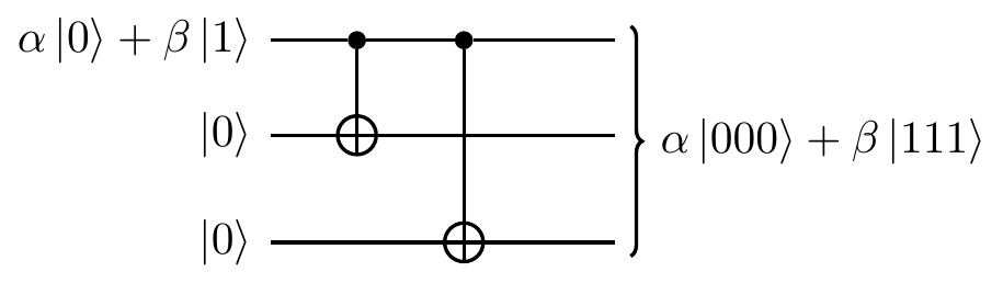
The result is the isometric embedding of the 2-dimensional Hilbert space of the first qubit (spanned by |0\rangle and |1\rangle) into the 2-dimensional subspace (spanned by |000\rangle and |111\rangle) of the 8-dimensional Hilbert space of the three qubits.
The isometric operator
V = |000\rangle\langle 0| + |111\rangle\langle 1|
acts via
\alpha|0\rangle+\beta|1\rangle
\longmapsto \alpha|000\rangle+\beta|111\rangle.
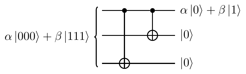
This three qubit-encoding can be reversed by the mirror image circuit:
This isometry is just one member of a family, and we will spend the rest of this chapter building up to the general theory, and understanding how this three-qubit encoding is useful in error correction.
Let’s start with the following scenario.
Alice constructs a quantum channel which is a mixture of four isometries.
The input is a single qubit, and the output is a dilated system composed of three qubits.
She prepares the input qubit in a state |\psi\rangle and then combines it with the two ancillary qubits which are in a fixed state |0\rangle|0\rangle.
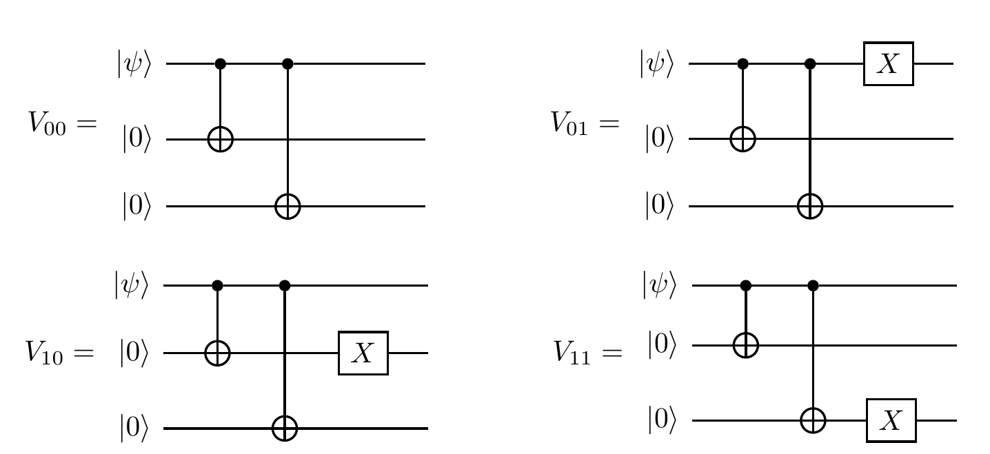
Then she applies one of the four, randomly chosen, unitary operations to the three qubits, to generate the following four isometries:
\begin{aligned}
V_{00} &= |000\rangle\langle 0| + |111\rangle\langle 1|
\\V_{01} &= |001\rangle\langle 0| + |110\rangle\langle 1|
\\V_{10} &= |010\rangle\langle 0| + |101\rangle\langle 1|
\\V_{11} &= |100\rangle\langle 0| + |011\rangle\langle 1|.
\end{aligned}
The three qubits, which form the output of the channel, are given to Bob, whose task is to recover the original state |\psi\rangle of the input qubit.
In this scenario, Bob, who knows the four isometries, can find out which particular isometry was applied.
He knows that
- V_{00} maps \mathcal{H} to \mathcal{H}'_{00}, which is a subspace of \mathcal{H}' spanned by |000\rangle and |111\rangle;
- V_{01} maps \mathcal{H} to \mathcal{H}'_{01}, which is a subspace of \mathcal{H}' spanned by |001\rangle and |110\rangle;
- V_{10} maps \mathcal{H} to \mathcal{H}'_{10}, which is a subspace of \mathcal{H}' spanned by |010\rangle and |101\rangle;
- V_{11} maps \mathcal{H} to \mathcal{H}'_{11}, which is a subspace of \mathcal{H}' spanned by |100\rangle and |011\rangle.
Given that these subspaces are mutually orthogonal, and \mathcal{H}'=\mathcal{H}'_{00}\oplus\mathcal{H}'_{01}\oplus\mathcal{H}'_{10}\oplus\mathcal{H}'_{11}, Bob can perform a measurement defined by the projectors on these subspaces.
For example, if Alice randomly picked V_{01}, then the input state |\psi\rangle=\alpha|0\rangle+\beta|1\rangle will be mapped to the output state \alpha|001\rangle+\beta|110\rangle in the \mathcal{H}'_{01} subspace.
Bob’s measurement
P_{01}
= |001\rangle\langle 001| + |101\rangle\langle 101|
will then detect \mathcal{H}'_{01} as the subspace where the output state resides, but the measurement (i.e. the corresponding projection) will not affect any state in that subspace.
Bob can now simply apply V_{01}^\dagger and obtain |\psi\rangle.
Below is a diagram of how the four isometries are implemented.
We will see how to reverse these operations in Section 13.2.