Single qubit interference
Let us now describe what is probably the most important sequence of operations performed on a single qubit: a generic single-qubit interference.
It is typically constructed as a sequence of three elementary operations:
- the Hadamard gate
- a phase-shift gate
- the Hadamard gate again.
We represent it graphically as
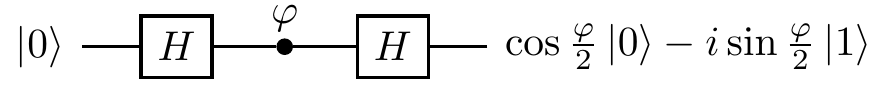
where the definitions of the Hadamard and phase-shift gates are as in Section 1.6:
| Hadamard |
H = \frac{1}{\sqrt{2}}\begin{bmatrix}1&1\\1&-1\end{bmatrix} |
\begin{array}{lcr}|0\rangle&\longmapsto&\frac{1}{\sqrt{2}}(|0\rangle+|1\rangle)\\|1\rangle&\longmapsto&\frac{1}{\sqrt{2}}(|0\rangle-|1\rangle)\end{array} |
| Phase-shift |
P_\varphi = \begin{bmatrix}1&0\\0&e^{i\varphi}\end{bmatrix} |
\begin{array}{lcr}|0\rangle&\longmapsto&|0\rangle\\|1\rangle&\longmapsto&e^{i\varphi}|1\rangle\end{array} |
Note that we sometimes use the notation |+\rangle and |-\rangle when talking about Hadamard gates, where
\begin{aligned}
|+\rangle &\coloneqq H|0\rangle = \frac{1}{\sqrt{2}}(|0\rangle+|1\rangle)
\\|-\rangle &\coloneqq H|1\rangle = \frac{1}{\sqrt{2}}(|0\rangle-|1\rangle).
\end{aligned}
You will see this specific sequence of gates over and over again, for it is quantum interference that gives quantum computation additional capabilities.
Something that many explanations of quantum computing say is the following: “quantum computers are quicker because they evaluate all possible solutions at once, in parallel”.
This is not accurate.
Firstly, quantum computers are not necessarily “quicker” than classical computers, but can simply implement quantum algorithms, some of which are quicker than their classical counterparts.
Secondly, the idea that they “just do all the possible computations at once” is false — instead, they rely on thoughtfully using interference (which can be constructive or destructive) to modify the probabilities of specific outcomes.
The motto to keep in mind is that the power of quantum computing comes from quantum interference.
The product of the three matrices HP_\varphi H describes the action of the whole circuit: it gives the transition amplitudes between states |0\rangle and |1\rangle at the input and the output as
\frac{1}{\sqrt{2}}
\begin{bmatrix}
1 & 1
\\1 & -1
\end{bmatrix}
\begin{bmatrix}
1 & 0
\\0 & e^{i\varphi}
\end{bmatrix}
\frac{1}{\sqrt{2}}
\begin{bmatrix}
1 & 1
\\1 & -1
\end{bmatrix}
= e^{i\frac{\varphi}{2}}
\begin{bmatrix}
\cos\varphi/2 & -i\sin\varphi/2
\\-i\sin\varphi/2 & \cos\varphi/2
\end{bmatrix}
Given that our input state is almost always |0\rangle, it is sometimes much easier and more instructive to step through the execution of this circuit and follow the evolving state.
The interference circuit effects the following sequence of transformations:
\begin{aligned}
|0\rangle
&\overset{H}{\longmapsto}
\frac{1}{\sqrt{2}} \left(
|0\rangle+|1\rangle
\right)
\\&\overset{P_\phi}{\longmapsto}
\frac{1}{\sqrt{2}} \left(
|0\rangle+e^{i\phi}|1\rangle
\right)
\\&\overset{H}{\longmapsto}
\cos\frac{\phi}{2}|0\rangle - i\sin\frac{\phi}{2}|1\rangle.
\end{aligned}
The first Hadamard gate prepares an equally weighted superposition of |0\rangle and |1\rangle and the second Hadamard closes the interference by bringing the interfering paths together.
The phase shift \varphi in between effectively controls the entire evolution and determines the output.
The probabilities of finding the qubit in state |0\rangle or |1\rangle at the output are, respectively,
\begin{aligned}
\Pr(0) &= \cos^2\frac{\phi}{2}
\\\Pr(1) &= \sin^2\frac{\phi}{2}.
\end{aligned}
This simple quantum process contains, in a nutshell, the essential ingredients of quantum computation.
This sequence (Hadamard–phase shift–Hadamard) will appear over and over again.
It reflects a natural progression of quantum computation: first we prepare different computational paths, then we evaluate a function which effectively introduces phase shifts into different computational paths, then we bring the computational paths together at the output.