3.1 Beam-splitters: physics against logic

A symmetric beam-splitter is a cube of glass which reflects half the light that impinges upon it, while allowing the remaining half to pass through unaffected. For our purposes it can simply be viewed as a device that has two input and two output ports, which we label with |0\rangle and |1\rangle as in Figure 3.1.

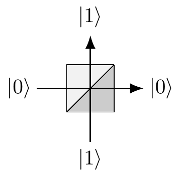
Figure 3.1: A symmetric beam-splitter, with input ports on the bottom and the left sides, and output ports on the top and the right sides.

When we aim a single photon at such a beam-splitter using one of the input ports, we notice that the photon doesn’t split in two: we can place photo-detectors wherever we like in the apparatus, fire in a photon, and verify that if any of the photo-detectors registers a hit, none of the others do. In particular, if we place a photo-detector behind the beam-splitter in each of the two possible exit beams, the photon is detected with equal probability at either detector, no matter whether the photon was initially fired into input port |0\rangle or |1\rangle.

If we fire the photon into the input port |0\rangle, it may seem obvious that, at the very least, the photon is either in the transmitted beam |0\rangle or in the reflected beam |1\rangle during any one run of this experiment. Thus we may be tempted to think of the beam-splitter as a random binary switch which, with equal probability, transforms any binary input into one of the two possible outputs. However, as you might expect (now having already learnt about the double-slit experiment), this is not necessarily the case. Let us introduce a second beam-splitter and place two normal mirrors so that both paths intersect at the second beam-splitter, as well as putting a detector at each output port of the second beam-splitter (see Figure 3.2).

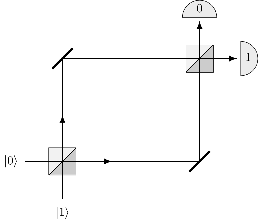
Figure 3.2: Two beam-splitters with mirrors, arranged so that the photon travels through both, along with two detectors. We label the detectors in such a way that, if a photon enters input |j\rangle and is transmitted (not reflected) through both beam-splitters, then it is detected by detector j.

Recall the Kolmogorov additivity axiom in classical probability theory: whenever something can happen in several alternative ways, we add probabilities for each way considered separately. We might argue that a photon fired into the input port |0\rangle can reach the detector 0 in two mutually exclusive ways: either by two consecutive reflections or by two consecutive transmissions. Each reflection happens with probability 1/2, and each transmission happens with probability 1/2, so the total probability of a photon fired into input |0\rangle reaching detector 0 is the sum of the probability of the two consecutive reflections (1/2\times 1/2 = 1/4) and the probability of the two consecutive transmissions (1/2\times 1/2 = 1/4), which gives a probability of 1/2. This is summarised in Figure 3.3, and makes perfect sense — a random switch followed by a random switch should give nothing else but a random switch.

However, if we set up such an experiment in a lab, this is not what happens!

There is no reason why probability theory (or any other a priori mathematical construct for that matter) should make any meaningful statements about outcomes of physical experiments.

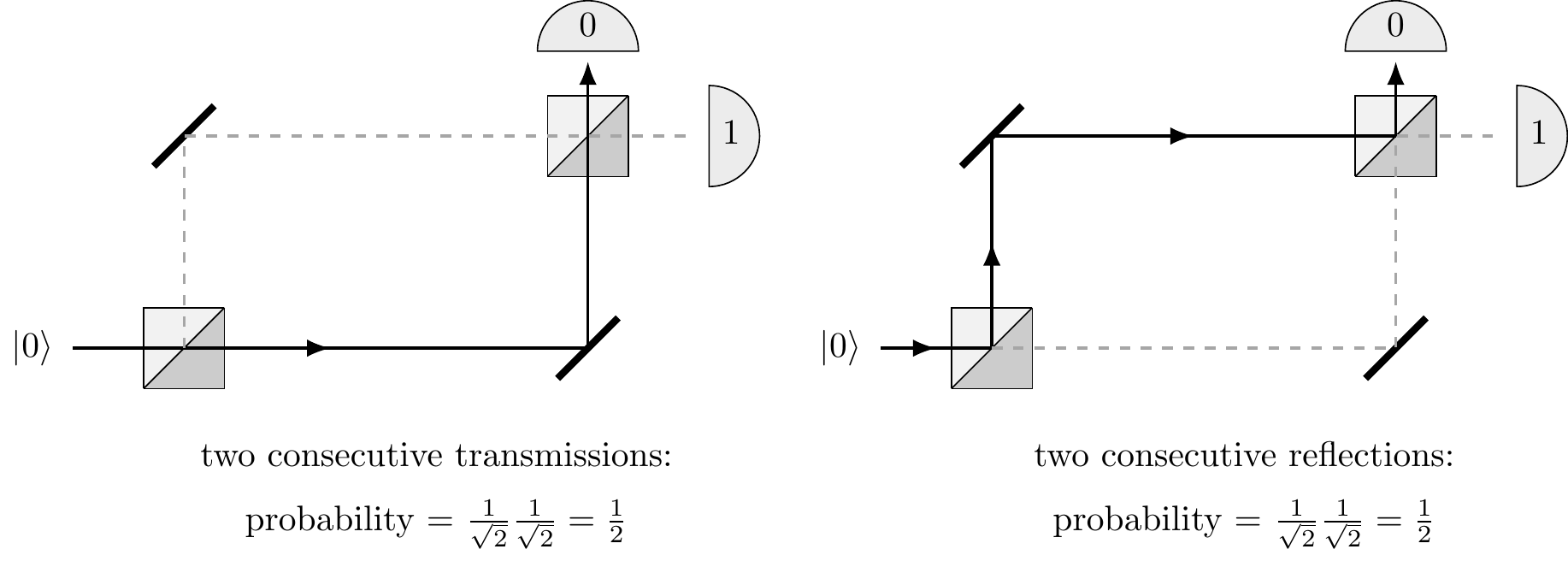
Figure 3.3: The two possible classical scenarios. Note that this is not what actually happens in the real physical world!

In experimental reality, when the optical paths between the two beam-splitters are the same, the photon fired from input port |0\rangle always strikes detector 1 and never detector 0 (and the photon fired from input port |1\rangle always strikes detector 0 and never detector 1). In other words, a beam-splitter is a physical implementation of a \sqrt{\texttt{NOT}} gate.

The action of the beam-splitter — in fact, the action of any quantum device — can be described by tabulating the amplitudes of transitions between its input and output ports.⁶⁶ B = \begin{bmatrix} B_{00} & B_{01}\\ B_{10} & B_{11} \end{bmatrix} = \begin{bmatrix} \frac{1}{\sqrt{2}} & \frac{i}{\sqrt{2}}\\ \frac{i}{\sqrt{2}} & \frac{1}{\sqrt{2}} \end{bmatrix}. The matrix element B_{lk}, where k,l=0,1, represents the amplitude of transition from input |k\rangle to output |l\rangle (watch the order of indices). Each reflection (entries B_{01} and B_{10}) happens with amplitude i/\sqrt{2}, and each transmission (entries B_{00} and B_{11}) happens with amplitude 1/\sqrt{2}. So the total amplitude that a photon fired from input port |0\rangle will reach detector 0 is the sum of the amplitude of the two consecutive reflections (i/\sqrt{2}\times i/{\sqrt{2}} = -1/2) and the amplitude of the two consecutive transmissions (1/{\sqrt{2}}\times 1/{\sqrt{2}} = 1/2) which gives the total amplitude 0, and thus a resulting probability of zero.

Unlike probabilities, amplitudes can cancel each other out, witnessing destructive interference.

We can now go on and calculate the amplitude that the photon will reach detector 1. In this case we will get i, which gives probability 1 (since |i|^2=1). We can then switch to input |1\rangle and repeat our calculations. All possible paths and associated amplitudes are shown in Figure 3.4.

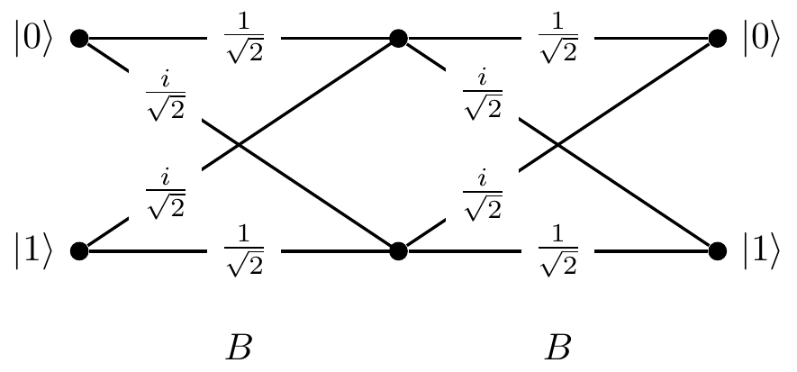
Figure 3.4: All possible transitions and their amplitudes when we compose two beam-splitters, as described by the matrix B above.

However, instead of going through all the paths in this diagram and linking specific inputs to specific outputs, we can simply multiply the transition matrices: BB = \begin{bmatrix} \frac{1}{\sqrt{2}} & \frac{i}{\sqrt{2}}\\ \frac{i}{\sqrt{2}} & \frac{1}{\sqrt{2}} \end{bmatrix} \begin{bmatrix} \frac{1}{\sqrt{2}} & \frac{i}{\sqrt{2}}\\ \frac{i}{\sqrt{2}} & \frac{1}{\sqrt{2}} \end{bmatrix} = \begin{bmatrix} 0 & i\\ i & 0 \end{bmatrix} = iX where X = \texttt{NOT}= \begin{bmatrix}0&1\\1&0\end{bmatrix}.

Bit-flip	\texttt{NOT}\equiv X	\begin{bmatrix}0&1\\1&0\end{bmatrix}
Beam-splitter	\sqrt{\texttt{NOT}}\equiv B	\frac{1}{\sqrt{2}}\begin{bmatrix}1&i\\i&1\end{bmatrix}

---

66. Note that gate B is not the same square root of \texttt{NOT} as the one we have already seen. In fact, there are infinitely many ways of implementing this “impossible” logical operation.↩︎