Hidden-order determination
In the same way that Deutsch’s algorithm (10.4) dealt with binary observable measurement for a unitary implementing some function evaluation, the hidden-order determination algorithm that we are now going to study deals with phase estimation for a unitary implementing some function evaluation.
This turns out to be an important step along the path towards Shor’s algorithm
(Hidden-order determination).
We are presented with an oracle that computes the function on n qubits
U_a|z\rangle
= |az\ \mathrm{mod}\ N\rangle
for some fixed (known) integer N=2^n, along with a fixed (known) integer a that is coprime to N.
Our task is to determine, using the fewest queries possible, the order r of a modulo N, i.e. the smallest positive integer r such that a^r\equiv1\ \mathrm{mod}\ N.
Let’s be clear and spell out what notational shortcuts we’re making here.
Every integer 0\leqslant z<2^n corresponds to a basis state |z\rangle of the space of n qubits, given by writing z in binary form.
So when we write |az\ \mathrm{mod}\ N\rangle, this means that we take the product of the integers a and z, take this integer modulo N, and then consider the basis state given by writing this result in binary form.
The hypothesis that N is a power of 2 is actually unnecessary, as we will later explain, but we assume it for now since for the sake of ease.
First of all, we can write down some eigenstates of U_a parametrised by an integer s\in\mathbb{Z}
|u_s\rangle
= \frac{1}{\sqrt{r}} \sum_{k=0}^{r-1} e^{-2\pi i({sk}/{r})} |a^k\ \mathrm{mod}\ N\rangle.
Since 2\pi i(r+1)k/r\equiv2\pi i(k/r)\ \mathrm{mod}\ 2\pi i, we see that this gives us r eigenstates, parametrised by s=0,\ldots,r-1
Now let’s show that these are indeed eigenstates.
By the definition of U_a,
\begin{aligned}
U_a |u_s\rangle
&= \frac{1}{\sqrt{r}}\sum_{k=0}^{r-1} e^{-2\pi i({sk}/{r})} |y^{k+1}\ \mathrm{mod}\ N\rangle
\\&= \frac{1}{\sqrt{r}}\sum_{j=1}^{r} e^{2\pi i({s}/{r})}e^{-2\pi i({sj}/{r})} |y^{j}\ \mathrm{mod}\ N\rangle
\end{aligned}
where we simply changed the index of the sum to j=k+1.
But r is the order of a modulo N, so we the j=r term can be written as j=0, giving
U_a |u_s\rangle
= e^{2\pi i({s}/{r})}|u_s\rangle
which shows that |u_s\rangle is an eigenstate with eigenvalue e^{2\pi i(s/r)}.
Of course, we cannot actually prepare any of these eigenstates |u_s\rangle because they require knowledge of the natural number r that we are trying to find!
But at the very least this now looks a bit like a problem that we have seen before: if we could prepare some particular |u_s\rangle then the phase estimation algorithm (from Section 10.8) would allow us to calculate s/r, and thus r.
So let’s try one of our always-useful tricks: superposition.
Although we cannot prepare any |u_s\rangle individually, note that
\begin{aligned}
\frac{1}{\sqrt{r}} \sum_{s=0}^{r-1} |u_s\rangle
&= \frac{1}{r} \sum_{s=0}^{r-1} \sum_{k=0}^{r-1} e^{-2\pi i({sk}/{r})} |a^k\ \mathrm{mod}\ N\rangle
\\&= \frac{1}{r} \sum_{k=0}^{r-1} \left(\sum_{s=0}^{r-1} e^{-2\pi i({sk}/{r})}\right) |a^k\ \mathrm{mod}\ N\rangle
\\&= \underbrace{\frac{1}{r} \sum_{s=0}^{r-1} |1\rangle}_{k=0} + \frac{1}{r} \sum_{k=1}^{r-1} \left(\sum_{s=0}^{r-1} e^{-2\pi i({sk}/{r})}\right) |a^k\ \mathrm{mod}\ N\rangle
\\&= |1\rangle
\end{aligned}
and so we should get something interesting by just plugging in |1\rangle.
The actual circuit is practically identical to the phase estimation circuit of Section 10.8, but where U is replaced by U_a, and |u\rangle is replaced by |1\rangle.
(Shor’s order-finding algorithm).
First register: 2n+1 qubits. Second register: n qubits.
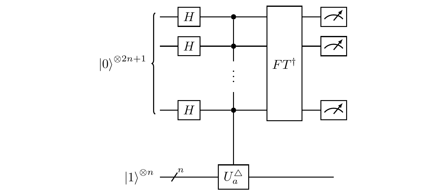
As always, let’s step through the circuit.
Immediately after the first Hadamard we are in the state
\left(\frac{1}{\sqrt{N}}\sum_{x=0}^{N-1}|x\rangle\right)|1\rangle.
Next, just after the function evaluation U_a, we are in the state
\frac{1}{\sqrt{r}} \sum_{s=0}^{r-1} |\Phi_s\rangle|u_s\rangle
where
|\Phi_s\rangle
= \frac{1}{\sqrt{N}} \sum_{n=0}^{N-1} e^{i\phi_s x}|x\rangle
and \phi_s=2\pi(s/r), so that e^{i\phi_s x} is the eigenvalue of |u_s\rangle for U_a.
To calculate the effect of the inverse quantum Fourier transform, we will make the same pedagogical shortcut as we did when studying Simon’s algorithm (Section 10.7) and pretend that we make a measurement in the basis |u_s\rangle in the auxiliary system before applying the inverse QFT.
We will measure one of the r possible values of s, each with equal probability 1/r, and doing so will leave the main register in the corresponding state |\Phi_s\rangle.
But this is exactly the picture of what happened after applying U^\triangle in the phase estimation circuit!
This means that we already know what the inverse QFT will do: it will give us the value of 2^{2n+1}(s/r).
Since this will happen irrelevant of which value of s we measure, we need not actually perform the measurement.
So running through the entire circuit and then measuring the main register will give us the value of 2^{2n+1}(s/r), which is almost enough to recover the value of r, but not quite: since we didn’t measure the auxiliary register, we don’t know which value of s we obtained!
However, now a purely classical (and efficient) algorithm comes to our rescue: the continued fractions algorithm.
This will give us the values of s and r provided that a certain inequality is satisfied, which is always the case if our main register has 2n+1 qubits.
We will not delve into these details of the classical post-processing of the measurements since they are no longer quantum; consider this yet another chance for the interested reader to either work out the details themselves or to find the answers elsewhere through some research of their own.
Finally, the assumption at the very start that N be of the form 2^n is not actually necessary (just as the assumption that the phase in the phase estimation problem be of the form 2\pi m/2^n is not actually necessary).
Suppose that N isn’t of this form, and let n be the smallest integer such that N<2^n.
Then we want to extend U_a to act on n qubits, and we need to be careful how we do so.
For example, we cannot simply take the same function U_a|z\rangle=|az\ \mathrm{mod}\ N\rangle, since then U_a|0\rangle=|0\rangle=U_a|N\rangle but |0\rangle and |N\rangle are orthogonal (remember, we always assume our bases to be orthonormal!), so this U_a cannot be unitary because it sends orthogonal states to non-orthogonal states.
The correct modification to make for our purposes is to define
U_a|z\rangle
= \begin{cases}
|az\ \mathrm{mod}\ N\rangle
& 0\leqslant z<N
\\|z\rangle
& R\leqslant z<2^n
\end{cases}
which is indeed unitary over the whole space of n qubits.