Simon’s algorithm
Here we will see the simplest quantum algorithm that offers an exponential speed-up when compared to the best possible classical algorithm.
(Hidden binary-addition determination).
We are presented with an oracle that computes some unknown function f\colon\{0,1\}^n\to\{0,1\}^n, but we are promised that f satisfies, for all x\in\{0,1\}^n,
f(x) = f(x\oplus s)
for some fixed s\in\{0,1\}^n, which we call the period of f.
(We assume that s is not the string of n zeros, otherwise the problem becomes trivial.)
Our task is to determine, using the fewest queries possible, the value of the n-bit string s.
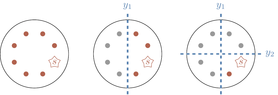
Note that asking for f to be periodic is equivalent to asking that f be two-to-one: for any y\in\{0,1\}^n such that there exists some x\in\{0,1\}^n with f(x)=y, there exists exactly one other x'\neq x such that f(x')=y as well.
Classically, this problem is exponentially hard.
We will not go through a detailed proof of this fact, but the intuition is reasonably simple: since there is no structure in the function f that would help us find its period s, the best we can do is evaluate f on random inputs and hope that we find some distinct x and x' such that f(x)=f(x'), and then we know that s=x\oplus y.
After having made m queries to the oracle, we have a list of m-many tuples (x,f(x)); there are m(m-1)/2 possible pairs which could match within this list, and the probability that a randomly chosen pair match is 1/2^{n-1}.
This means that the probability of there being at least one matching pair within the list of m tuples is less than m^2/2^n.
This means that the chance of finding a matching pair is negligible if the oracle is queried on fewer than m=\sqrt{2^n} inputs.
The quantum case, on the other hand, gives a result (again, with “high” probability) within a linear number of steps.
The circuit that solves this problem, shown below, has a familiar Hadamard–function–Hadamard structure, but the second register has now been expanded to n qubits.
First register: n qubits. Second register: n qubits.
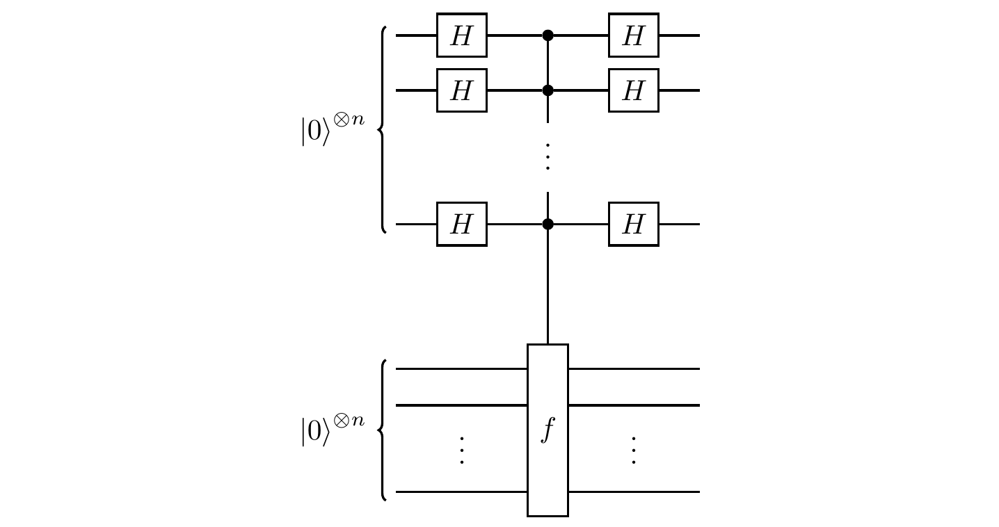
This time, let’s follow the evolution of both registers throughout this circuit.
We start off by preparing the equally-weighted superposition of all n-bit strings with the first Hadamard, and then query the oracle:
\begin{aligned}
|0^{\otimes n}\rangle|0^{\otimes n}\rangle
&\overset{H^{\otimes n}\otimes\mathbf{1}}{\longmapsto}
\frac{1}{\sqrt{2^n}} \sum_x |x\rangle|0^{\otimes n}\rangle
\\&\overset{U_f}{\longmapsto}
\frac{1}{\sqrt{2^n}} \sum_x |x\rangle|f(x)\rangle.
\end{aligned}
The second Hadamard transform on the first register then yields the final output state:
\frac{1}{2^n} \sum_{x,y} (-1)^{x\cdot y} |y\rangle|f(x)\rangle.
\tag{$\ddagger$}
But if we measure the second register before applying the second Hadamard transform to the first register, we obtain one of the 2^{n-1} possible values of f(x), each equally likely.
Let’s study the implications of this.
Suppose that the outcome of the measurement is f(a) for some a\in\{0,1\}^n.
Given that both a and a\oplus s are mapped to f(a) by f, the first register then collapses to the state
\frac{1}{\sqrt{2}}\big( |a\rangle + |a\oplus s\rangle \big).
The subsequent Hadamard transform on the first register then gives us the final state
\begin{aligned}
&\frac{1}{\sqrt{2^{n+1}}} \sum_y \Big((-1)^{a\cdot y}+(-1)^{(a\oplus s)\cdot y}\Big) |y\rangle|f(a)\rangle
\\= &\frac{1}{\sqrt{2^{n+1}}} \sum_y (-1)^{a\cdot y}
\Big( 1 + (-1)^{s\cdot y} \Big) |y\rangle|f(a)\rangle
\\= &\frac{1}{\sqrt{2^{n-1}}} \sum_{y\in s^\perp}
(-1)^{a\cdot y} |y\rangle|f(a)\rangle
\end{aligned}
where we have used the fact that (a\oplus s)\cdot y = (a\cdot y)\oplus(s\cdot y), and that 1+(-1)^{s\cdot y} can have only two values: either 2 (when s\cdot y = 0) or 0 (when s\cdot y = 1).
Now we finally measure the first register: the outcome is selected at random from all possible values of y such that s\cdot y = 0, each occurring with probability 1/(2^{n-1}).
In fact, we did not have to measure the second register at all: it was a mathematical shortcut, simply taken for pedagogical purposes.
Instead of collapsing the state to just one term in a superposition, we can express Equation (\ddagger) as
\begin{aligned}
&\frac{1}{2^n} \sum_{y,f(a)}
\Big( (-1)^{a\cdot y} + (-1)^{(a\oplus s)\cdot y} \Big) |y\rangle|f(a)\rangle
\\= &\frac{1}{2^n} \sum_{y,f(a)} (-1)^{a\cdot y}
\Big( 1 + (-1)^{s\cdot y} \Big) |y\rangle|f(a)\rangle
\end{aligned}
where the summation over f(a) means summing over all binary strings in the image of f, which is a convenient shorthand for the more complicated formal statement: for all z\in\{0,1\}^n, since our function f is two-to-one, we know that the preimage f^{-1}(z) has either two elements or none; if it’s the latter, then we don’t include z in our sum; if it’s the former, we pick one and call it a (knowing that the other, by the setup, must be a\oplus s, which you can see appearing in the first equation above).
With this, the final output of the algorithm is
\frac{1}{2^{n-1}} \sum_{y\in s^\perp} |y\rangle
\sum_{f(a)} (-1)^{a\cdot y} |f(a)\rangle
and, again, the measurement outcome is selected at random from all possible values of y such that s\cdot y=0.
We are not quite done yet: we cannot infer s from a single output y.
However, once we have found n-1 linearly independent strings y_1,y_2,\ldots,y_{n-1}, we can solve the n-1 equations
\left\{
\begin{aligned}
s\cdot y_1 &= 0
\\s\cdot y_2 &= 0
\\&\,\,\,\vdots
\\s\cdot y_{n-1} &= 0
\end{aligned}
\right\}
to determine a unique value of s.
(Note that we only need n-1 values, and not n, because s=0 will always be a solution, but we have explicitly assumed that this is not the case in our statement of the scenario, and so it suffices to narrow down the space of possible solutions to consist of two elements, since then we know that we can just take the non-zero one.)
So we run this algorithm repeatedly, each time obtaining another value of y that satisfies s\cdot y = 0.
Every time we find some new value of y that is linearly independent of all previous ones, we can discard half the potential candidates for s.
Now, the probability that (n-1)-many outputs y_1,\ldots,y_{n-1} are linearly independent is
\left( 1-\frac{1}{2^{n-1}} \right)
\left( 1-\frac{1}{2^{n-2}} \right)
\ldots
\left( 1-\frac{1}{2} \right).
\tag{$\circledast$}
To see this, suppose that we have k linearly independent binary strings y_1,\ldots,y_k.
Then these strings span a subspace with 2^k elements, consisting of all binary strings of the form \bigoplus_{i=1}^k b_i y_i, where b_1,\ldots,b_k\in\{0,1\}.
Now suppose we obtain some y_{k+1}.
It will be linearly independent from the y_1,\ldots,y_k if and only if it lies outside the subspace spanned by the y_1,\ldots,y_k, which occurs with probability 1-(2^k)/(2^n).
We can bound Equation (\circledast) from below:
the probability of obtaining a linearly independent set \{y_1,\ldots,y_{n-1}\} by running the algorithm n-1 times (i.e. not having to discard any values and run again) is
\prod_{k=1}^{n-1}
\left(
1-\frac{1}{2^k}
\right)
\geqslant
\left[
1 -
\left(
\frac{1}{2^{n-1}} + \frac{1}{2^{n-2}} + \ldots + \frac{1}{4}
\right)
\right]
\cdot \frac{1}{2}
>
\frac{1}{4}.
We conclude that we can determine s with some constant probability of error after repeating the algorithm \mathcal{O}(n) times.
The exponential separation that this algorithm demonstrates between quantum and classical highlights the vast potential of a quantum computer to speed up function evaluation.