Grover’s search algorithm
The next algorithm we will study aims to solve the problem of searching for a specific item in an unsorted database.
Think about an old-fashioned phone book: the entries are typically sorted alphabetically, by the name of the person that you want to find.
However, what if you were in the opposite situation: you had a phone number and wanted to find the corresponding person’s name?
The phone book is not sorted in that way, and to find the number (and hence name) with, say, 50% probability, you would need to search through, on average, 50% of the entries.
Needless to say, in a large phone book this would take a long time.
While this might seem like a rather contrived problem (a computer database should always maintain an index on any searchable field), many problems in computer science can be cast in this form, i.e. that of an unstructured search.
We are presented with an oracle that computes some unknown function f\colon\{0,1\}^n\to\{0,1\}.
Our task is to find, using the fewest queries possible, an input x\in\{0,1\}^n such that f(x)=1.
Suppose that we know that, amongst the N=2^n binary strings, there are M\ll N which are tagged, i.e. strings on which f evaluates to 1.
Since there is no structure in the database, any classical search requires around N/M steps, i.e. the function f must be evaluated roughly N/M times.
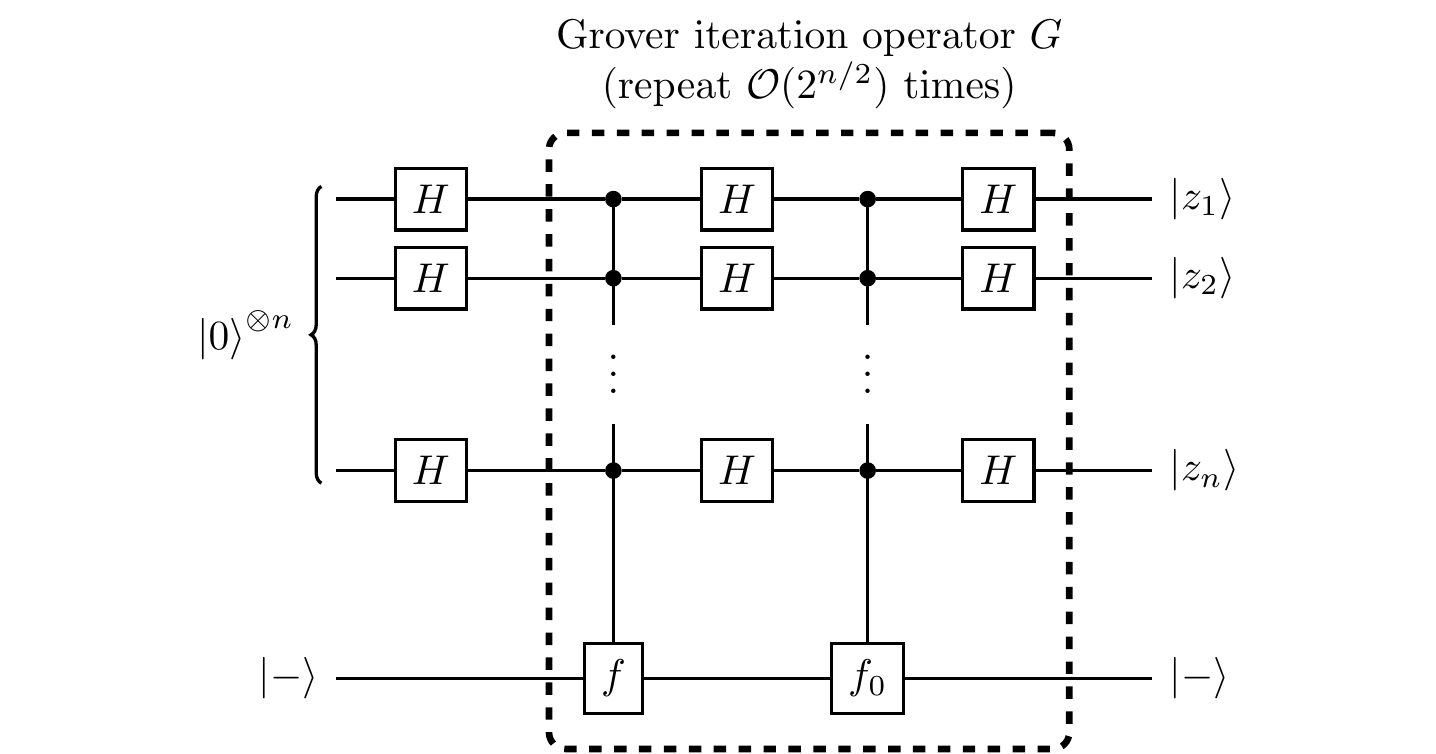
In contrast, there is a quantum search algorithm, implemented by the circuit below, which requires only roughly \sqrt{N/M} steps.
First register: n qubits. Second register: 1 qubit.
where f_0 tags the binary string consisting of n zeros:
f_0(x)
= \begin{cases}
1 &\text{if $x=00\ldots0$;}
\\0 &\text{otherwise.}
\end{cases}
Yet again, we can recognise the typical Hadamard, function evaluation, Hadamard sequence, and yet again we can see that the second register (the bottom qubit, in state |-\rangle) plays an auxiliary role: the real action takes place in the first register.
However, unlike the previous algorithms, a single call to the oracle does not do very much, and we have to build up the quantum interference in the first register through repeated calls to the oracle (without any intermediate measurements!).
Here, the basic step is the Grover iteration operator G, which is the boxed part of the circuit that we repeat over and over:
G = (H^{\otimes n}\otimes\mathbf{1}) U_{f_0}(H^{\otimes n}\otimes\mathbf{1}) U_f.
After \mathcal{O}(2^{n/2}) applications of G, we measure the first register bit-by-bit and obtain the value of |z\rangle=|z_1z_2\ldots z_n\rangle, which is such that, with “high” probability, f(z)=1.
In order to actually see how this algorithm works, and to justify our use of the phrase “with high probability”, we can take a more geometric approach.
First, we define two orthonormal vectors in the Hilbert space describing the first register:
\begin{aligned}
|a\rangle
&= \frac{1}{\sqrt{N-M}} \sum_{x\in f^{-1}(0)} \!\!\!\!|x\rangle
\\|b\rangle
&= \frac{1}{\sqrt{M}} \sum_{x\in f^{-1}(1)} \!\!\!\!|x\rangle
\end{aligned}
where f^{-1}(i)\coloneqq\{x\in\{0,1\}^n\mid f(x)=i\} is the preimage of i.
Since these vectors are orthonormal, they are, in particular, linearly independent, and so their span is a two-dimensional subspace — this is the subspace in which our search will take place.
Using the fact that f^{-1}(0) and f^{-1}(1) form a partition of the space \{0,1\}^n, we see that the two-dimensional span of |a\rangle and |b\rangle contains, in particular, the equally-weighted superposition |s\rangle=H^{\otimes n}|0^{\otimes n}\rangle of all binary strings of length n:
\begin{aligned}
|s\rangle
&= \frac{1}{\sqrt{N}}\sum_{x\in\{0,1\}^n}|x\rangle
\\&= \frac{1}{\sqrt{N}}\sum_{x\in f^{-1}(0)}|x\rangle + \frac{1}{\sqrt{N}}\sum_{x\in f^{-1}(1)}|x\rangle
\\&= \sqrt{\frac{N-M}{N}}|a\rangle + \sqrt{\frac{M}{N}}|b\rangle
\\&= (\cos\theta)|a\rangle + (\sin\theta)|b\rangle
\end{aligned}
where we use the fact that
\sqrt{\frac{N-M}{N}}^2 + \sqrt{\frac{M}{N}}^2
= 1
= \sin^2\theta+\cos^2\theta
to parametrise \sqrt{\frac{N-M}{N}} as \cos\theta and \sqrt{\frac{M}{N}} as \sin\theta (with \theta\approx\sqrt{\frac{M}{N}}, since N\gg M).
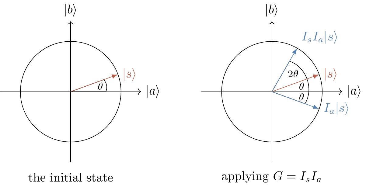
The state |s\rangle is our starting input for our sequence of Grover iterations, and we will show that applying G, when restricting to the plane spanned by |a\rangle and |b\rangle, amounts to applying a rotation by angle 2\theta.
Grover’s search algorithm can then be understood as a sequence of rotations which take the input state |s\rangle towards the target state |b\rangle.
To see this, note that the unitary transformation induced by the oracle
f\colon |x\rangle \mapsto (-1)^{f(x)}|x\rangle
can be written as
I_a \coloneqq 2|a\rangle\langle a|-\mathbf{1}
which we can interpret as a reflection through the |a\rangle-axis: we see that
\begin{aligned}
I_a|a\rangle
&= 2|a\rangle\langle a||a\rangle-|a\rangle
\\&= 2|a\rangle-|a\rangle
\\&= |a\rangle
\\I_a|b\rangle
&= 2|a\rangle\langle a||b\rangle-|b\rangle
\\&= -|b\rangle
\end{aligned}
and since -|b\rangle is a vector that points in the opposite direction from |b\rangle, it must be a reflection; since -|b\rangle is still orthogonal to |a\rangle, the reflection must be in the |a\rangle-axis.
Some further algebraic manipulation shows that I_a = 2|a\rangle\langle a|-\mathbf{1}= \mathbf{1}-2|b\rangle\langle b|.
Now, in particular, evaluation of f_0 can be written as 2|0\rangle\langle 0|-\mathbf{1}, and thus thought of as a reflection through the |0\rangle-axis.
If we sandwich f_0 in between two Hadamards then we obtain I_s = 2|s\rangle\langle s|-\mathbf{1}, which is reflection through the |s\rangle-axis.
By definition then, the Grover iteration operator G is the composition
G = I_s I_a.
Now recall the purely geometric fact that if we have two intersecting lines L_1 and L_2 in two-dimensional Euclidean space, meeting with angle \alpha, then reflecting an object through L_1 and then reflecting the resulting image through L_2 is the same as simply rotating the original object around the point of intersection L_1\cap L_2 by an angle of 2\alpha.
The angle between |a\rangle and |s\rangle is \theta, so each time G is applied the vector is rotated (around the origin) by an angle of 2\theta towards the |b\rangle-axis.
All that remains to do is to just choose the “right” number r of steps such that we end up as close to the |b\rangle-axis as possible.
The state |s\rangle starts at angle \theta to |a\rangle, and we should perform our final (and only) measurement when this angle is \pi/2, i.e. when (2r+1)\theta = \pi/2, which gives
r \approx \frac{\pi}{4}\sqrt{\frac{N}{M}}.
So the quantum algorithm searches an unsorted list of N items in roughly \sqrt{N} steps: it offers a quadratic speed-up when compared to classical search, which can be of immense practical importance.
For example, cracking some of the more popular modern ciphers, such as AES, essentially requires a search among many binary strings (called keys).
If these can be checked at a rate of, say, one million keys per second, then a classical computer would need over a thousand years to find the correct key, while a quantum computer using Grover’s algorithm would find it in less than four minutes.