Partial trace, revisited
You can calculate the trace of a matrix by summing its diagonal entries.
Can you do something similar to calculate the partial trace of a density matrix?
Suppose someone writes down for you a density matrix of two qubits in the standard basis, \{|00\rangle, |01\rangle, |10\rangle, |11\rangle\}, and asks you to find the reduced density matrices of the individual qubits.
The tensor product structure of this (4\times 4) matrix means that it is has a block form:
\rho_{\mathcal{AB}}
= \left[
\begin{array}{c|c}
P & Q
\\\hline
R & S
\end{array}
\right]
where P,Q,R,S are (2\times 2) sized sub-matrices.
The two partial traces can then be evaluated as
\begin{aligned}
\rho_{\mathcal{A}}
&=
\operatorname{tr}_{\mathcal{B}}\rho_{\mathcal{AB}}
= \left[
\begin{array}{c|c}
\operatorname{tr}P & \operatorname{tr}Q
\\\hline
\operatorname{tr}R & \operatorname{tr}S
\end{array}
\right]
\\\rho_{\mathcal{B}}
&= \operatorname{tr}_{\mathcal{A}}\rho_{\mathcal{AB}}
= P+S.
\end{aligned}
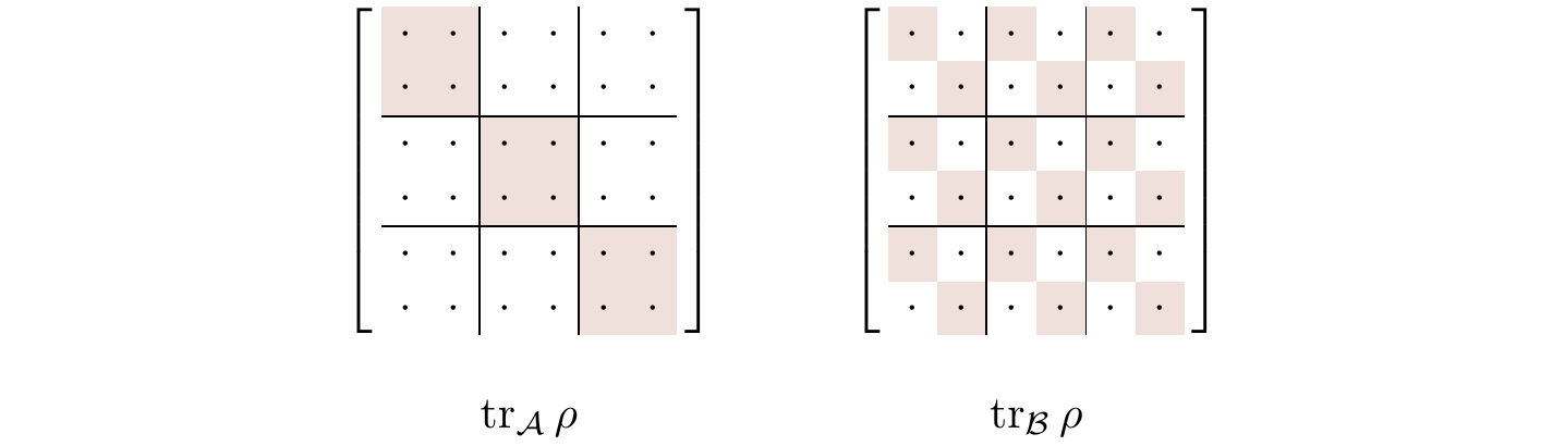
In general, for any matrix \rho in \mathcal{H}_{\mathcal{A}}\otimes\mathcal{H}_{\mathcal{B}} that is written in the tensor product basis, the partial trace over \mathcal{A} is the sum of the diagonal block matrices, and the partial trace over \mathcal{B} is the matrix in which the block sub-matrices are replaced by their traces — see Figure 8.1.
To better understand the partial trace, it helps to give a more abstract definition.
It turns out that the partial trace over \mathcal{B} can be defined as the unique map \rho_{\mathcal{AB}}\mapsto\rho_{\mathcal{A}} such that
\operatorname{tr}[X\rho_{\mathcal{A}}] = \operatorname{tr}[(X\otimes\mathbf{1})\rho_{\mathcal{AB}}]
\tag{$\circledast$}
holds for any observable X acting on \mathcal{A}, where \mathbf{1} is the identity operator acting on \mathcal{B}.
This condition ensures the consistency of statistical predictions: any observable X on \mathcal{A} can be viewed as an observable X\otimes\mathbf{1} on the composite system \mathcal{AB}; when constructing \rho_{\mathcal{A}}, we had better make sure that for any observable X the average value of X in the state \rho_{\mathcal{A}} is the same as the average value of X\otimes\mathbf{1} in the state \rho_{\mathcal{AB}}.
This is exactly what the condition in (\circledast) guarantees.
To show that our more ad-hoc definition of the partial trace agrees with this slightly more abstract one, consider again some state |\psi_{\mathcal{AB}}\rangle written in the form
\begin{aligned}
|\psi_{\mathcal{AB}}\rangle
&= \sum_{i,j} c_{ij}|a_i\rangle\otimes|b_j\rangle
\\&= \sum_{j} |\widetilde\psi_j\rangle|b_j\rangle
= \sum_{j} \sqrt{p_j}|\psi_j\rangle|b_j\rangle.
\end{aligned}
Now assume that Alice measures some observable X on her part of the system.
Such an observable can be thought of as X\otimes\mathbf{1}, acting on the entire system.
The expected value of this observable in the state |\psi_{\mathcal{AB}}\rangle is, by definition, \operatorname{tr}(X\otimes\mathbf{1})|\psi_{\mathcal{AB}}\rangle\langle\psi_{\mathcal{AB}}|, and
\begin{aligned}
\operatorname{tr}[(X\otimes \mathbf{1}) \rho_{\mathcal{AB}}]
&= \operatorname{tr}\left[
(X\otimes\mathbf{1}) \left(
\sum_{i,j} |\widetilde\psi_i\rangle\langle\widetilde\psi_j| \otimes |b_i\rangle\langle b_j|
\right)
\right]
\\&= \sum_{i,j} \left[
\operatorname{tr}\left(X |\widetilde\psi_i\rangle\langle\widetilde\psi_j|\right)
\right]
\underbrace{\left[\operatorname{tr}\left(|b_i\rangle\langle b_j|\right)\right]}_{\delta_{ij}}
\\&= \sum_i \operatorname{tr}\big[X |\widetilde\psi_i\rangle\langle\widetilde\psi_i|\big]
\\&= \operatorname{tr}\left[
X \underbrace{\sum_i p_i|\psi_i\rangle\langle\psi_i|}_{\rho_{\mathcal{A}} = \operatorname{tr}_{\mathcal{B}}\rho_{\mathcal{AB}}}
\right]
\\&= \operatorname{tr}[X\rho_{\mathcal{A}}]
\end{aligned}
as required.
We can also quickly prove why the partial trace is the unique map satisfying the condition (\circledast).
Suppose that we had some arbitrary map T satisfying this condition, i.e. such that
\operatorname{tr}[XT(\rho_{\mathcal{AB}})] = \operatorname{tr}[(X\otimes\mathbf{1})\rho_{\mathcal{AB}}]
for all density matrices \rho_{\mathcal{AB}} and for all observables X acting on \mathcal{A}.
Now, take some orthonormal (with respect to the Hilbert–Schmidt inner product (A|B)=\frac{1}{2}\operatorname{tr}A^\dagger B) basis \{M_i\} of the space of Hermitian matrices.
Since the M_i are Hermitian, the inner product (M_i|T(\rho_{\mathcal{AB}})) is just \operatorname{tr}[M_iT(\rho_{\mathcal{AB}})].
So when we expand T(\rho_{\mathcal{AB}}) in this basis we get
\begin{aligned}
T(\rho_{\mathcal{AB}})
&= \sum_i (M_i|T(\rho_{\mathcal{AB}})) M_i
\\&= \sum_i \operatorname{tr}[M_iT(\rho_{\mathcal{AB}})] M_i.
\end{aligned}
But now we can substitute in the condition that T satisfies, giving
T(\rho_{\mathcal{AB}})
= \sum_i \operatorname{tr}[(M_i\otimes\mathbf{1})\rho_{\mathcal{AB}}] M_i.
And we’re done!
Indeed, if we had started with some other such map T' then we would have arrived at the same expression, which is independent of our choice of T or T', whence T=T'.