Distinguishing non-orthogonal states, again
Let’s briefly return to the problem considered in Section 4.9, where we are given a system and told that it is in either state |\psi_1\rangle or |\psi_2\rangle, with equal probability, but that these two vectors are not orthogonal.
The goal is to find a measurement that maximises the probability of correctly identifying which state the system is in.
Before solving this problem using the language of distances, let us repeat the geometric idea that we used previously.
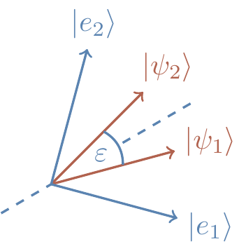
Draw two vectors, |\psi_1\rangle and |\psi_2\rangle, separated by some angle \varepsilon.
We want to find some orthonormal vectors |e_1\rangle and |e_2\rangle that specify the optimal projective measurement.
First, note that any projections on the subspace orthogonal to the plane spanned by |\psi_1\rangle and |\psi_2\rangle will reveal no information about the identity of the state, so we know that we will want our orthonormal vectors to lie in the span of |\psi_1\rangle and |\psi_2\rangle.
Now, since |\psi_1\rangle and |\psi_2\rangle are both equally likely to occur, we want to place |e_1\rangle and |e_2\rangle symmetrically around them, as shown in Figure 12.2
The probability of correctly distinguishing the two states is
p_{\mathrm{success}}
= \frac{1}{2}|\langle e_1|\psi_1\rangle|^2 + \frac{1}{2}|\langle e_2|\psi_2\rangle|^2
which reduces, with our schema, to
\begin{aligned}
p_{\mathrm{success}}
&= \cos^2\left(\frac{\pi}{2}-\frac{\varepsilon}{2}\right)
\\&= \frac{1}{2}(1+\sin\varepsilon)
\\&\approx \frac{1}{2}(1+\varepsilon)
\\&= \frac{1}{2}(1+\|\psi_1-\psi_2\|).
\end{aligned}
where the last equality holds whenever \varepsilon is “small enough”.
But, happily, we can be much more precise than this!
Let’s start by rephrasing the problem in terms of density operators.
We are sent one of two quantum states, either \rho_0 or \rho_1, with equal probability.
You might notice that we’re now labelling our states with \{0,1\} instead of \{1,2\}.
This is simply to help guide our intuition: we are being sent one bit of information, a 0 or a 1; the only complication is that this is happening in such a way that we cannot perfectly distinguish between them (since we are receiving non-orthogonal quantum states).
We want to choose two orthogonal projectors P_0 and P_1, so outcome P_0 is interpreted as a 0 and outcome P_1 as a 1.
The probability of correctly detecting which state was sent is, as always, the probability that \rho_0 was sent and outcome P_0 was observed, plus the probability that \rho_1 was sent and outcome P_1 was observed.
In symbols,
\begin{aligned}
p_{\mathrm{success}}
&= \frac{1}{2}\operatorname{tr}(P_0\rho_0) + \frac{1}{2}\operatorname{tr}(P_1\rho_1)
\\&= \frac{1}{4}\operatorname{tr}[(P_0+P_1)(\rho_0+\rho_1)] + \frac{1}{4}\operatorname{tr}[(P_0-P_1)(\rho_0-\rho_1)]
\\&= \frac{1}{2} + \frac{1}{4}\operatorname{tr}[(P_0-P_1)(\rho_0-\rho_1)]
\end{aligned}
where the last equality follows from the fact that P_0+P_1=\mathbf{1}.
By applying Hölder’s inequality, this tells us that
\begin{aligned}
p_{\mathrm{success}}
&\leqslant\frac{1}{2} + \frac{1}{4}\|(P_0-P_1)\|\|(\rho_0-\rho_1)\|_{\operatorname{tr}}
\\&\leqslant\frac{1}{2} + \frac{1}{4}\|\rho_0-\rho_1\|_{\operatorname{tr}}
\\&= \frac{1}{2}(1+d_{\operatorname{tr}}(\rho_0,\rho_1)).
\end{aligned}
Again, this upper bound is attained by taking P_0 to be the projector onto the eigenspace of \rho_0-\rho_1 corresponding to the positive eigenvalues, and P_1 the projector corresponding to the negative eigenvalues: this gives \operatorname{tr}(P_0-P_1)(\rho_0-\rho_1)=\|\rho_0-\rho_1\|_{\operatorname{tr}}.
Of course, the whole story of quantum state distinguishability has much more to it than we have covered here.
In Exercise 12.11.9 we ask about the case where the two states \rho_0 and \rho_1 are sent with non-equal probabilities p_0 and p_1, respectively.
The more general scenario, where some quantum source emits states \rho_0,\ldots,\rho_n with respective probabilities p_0,\ldots,p_n, turns out to be incredibly difficult — we do not know an optimal discrimination strategy, except for in a few special cases.