14.7 Error-correcting conditions

We can summarise the notion of a stabiliser code that we have defined rather succinctly: everything is determined by picking a stabiliser group, i.e. an abelian subgroup \mathcal{S} of the Pauli group \mathcal{P}_n that does not contain -\mathbf{1}. From this, we define the codespace to be the stabiliser subspace V_\mathcal{S}, the codewords to be a choice of basis vectors, the logical operators to be the cosets of \mathcal{S}\triangleleft N(\mathcal{S}), and the error families to be the cosets of N(\mathcal{S})\triangleleft\mathcal{P}_n.

By setting up some ancilla qubits and constructing appropriate quantum circuits³⁰⁵, we can enact any logical operator in such a way that we also measure an error syndrome, which points at a specific error family. But unlike in our study of the Steane code in Section 14.3, we can no longer simply apply the corresponding operator to fix the error, because the error is a whole coset — it contains many individual Pauli operators.

To fix an example to keep in mind, we return yet again to the three-qubit code. In Figure 14.8 we draw a diagram grouping together all the elements of \mathcal{P}_3 into the coset structure induced by \mathcal{S}=\langle ZZ\mathbf{1},\mathbf{1}ZZ\rangle. This is analogous to the diagrams that we saw back in Exercise 7.8.2, but with the simplification of ignoring phase.³⁰⁶

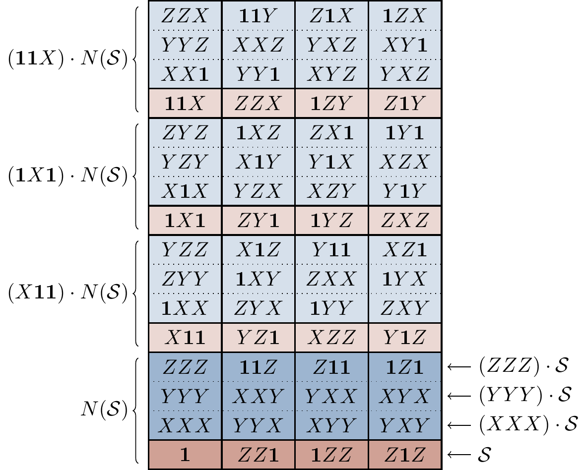
Figure 14.8: The entire group \mathcal{P}_3 with the coset structure induced by the stabiliser group \mathcal{S}=\langle ZZ\mathbf{1},\mathbf{1}ZZ\rangle. Note that we are ignoring global phase.

As we can see by looking at Figure 14.8, if we somehow measure an error syndrome pointing to the error family [X\mathbf{1}\mathbf{1}], for example, then there are 16 possible errors that could have occurred! We said that the stabiliser formalism would be better than our previous approach, so why do things seem so much worse now? Well, we are forgetting one key assumption that we made before that we have yet to impose in the stabiliser formalism: up until now, we have only studied single-qubit errors. Thinking back to our introduction of the three-qubit code in Section 13.1, we were specifically trying to deal with single bit-flip errors, i.e. only X\mathbf{1}\mathbf{1}, \mathbf{1}X\mathbf{1}, and \mathbf{1}\mathbf{1}X (as well as the trivial error \mathbf{1}\mathbf{1}\mathbf{1}, which we must not forget about, as we shall see). If we look back at Figure 14.8 with this in mind, we notice something particularly nice: each of these single X-type errors lives in a different error family, and each error family contains exactly one of these errors.

In other words, if we assume that only single bit-flip errors can occur, then the stabiliser formalism describes errors in exactly the same way as before, since the error families are in bijection with the physical errors. But here is where the power of the stabiliser formalism can really shine through, since it allows us to understand what type of error scenarios our code can actually deal with in full generality. That is, rather than thinking about a code as something being built to correct for a specific set of errors, the stabiliser formalism lets us say “here is a code”, and then ask “for which sets of errors is this code actually useful?”. The answer to this question lies in understanding how any set of physical errors is distributed across the error families, and we can draw even simpler versions of the diagram in Figure 14.8 to figure this out.

Returning to the scenario where we assume that only single bit-flip errors can occur, we can mark the corresponding physical errors in Figure 14.8 — namely \mathbf{1}, X\mathbf{1}\mathbf{1}, \mathbf{1}X\mathbf{1}, and \mathbf{1}\mathbf{1}X — with a dot. We do this in Figure 14.9, which is the first of many more diagrams of this form, which we call error-dot diagrams. Although we are working with the specific example of the three-qubit code in mind, these diagrams are meant to be understood more generally as applying to any stabiliser code. As we shall soon see, we don’t really need to worry about making sure that we have the right number of rows in each small rectangle (i.e. the right number of cosets of \mathcal{S} inside N(\mathcal{S})), and in some sense we don’t even really need to worry about what the physical errors are.

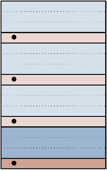
Figure 14.9: All specific X-type errors of weight at most 1 from Figure 14.8, each marked by a dot. The four cosets corresponding to N(\mathcal{S})\triangleleft\mathcal{P}_n are the error families, and we informally refer to the (copy of the) four cosets corresponding to \mathcal{S}\triangleleft N(\mathcal{S}) as rows.

As we said above, if each error family (i.e. coset) contains exactly one physical error (i.e. Pauli operator), then we already know how to apply corrections based on the error-syndrome measurements. In terms of the diagram in Figure 14.9, this rule becomes rather simple: if each error family contains exactly one dot, then we can error correct.

But can we say something more interesting than this? Well, let’s consider what happens if we have a diagram that looks like this:

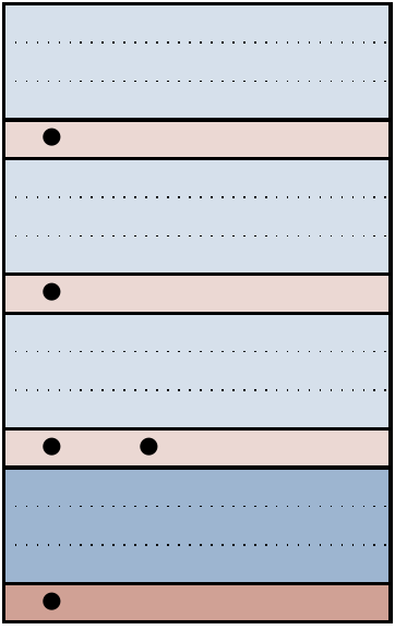
That is, we’re considering a scenario where there are two possible physical errors that can occur for a physical error syndrome. In the example of the three-qubit code, we’re looking at the scenario where any single bit-flip error can occur, but also the operator YZ\mathbf{1} might affect our computation, enacting a bit-phase-flip on the first qubit and a phase-flip on the second. What would then happen if we measured the error syndrome |01\rangle? We know (from Section 13.7) that this corresponds to the error family [X\mathbf{1}\mathbf{1}], but both X\mathbf{1}\mathbf{1} and YZ\mathbf{1} live in this coset, so we’re back to the question posed at the end of Section 14.5: how do we pick which operator to use to correct the error?

Here’s the fantastic fact: in this case, it doesn’t matter! Say we pick X\mathbf{1}\mathbf{1}, but the physical error that had actually affected our qubits, originally in some encoded state |\psi\rangle, was YZ\mathbf{1}. Then by applying the “correction” X\mathbf{1}\mathbf{1} our qubits would be in the state (X\mathbf{1}\mathbf{1})(YZ\mathbf{1})|\psi\rangle = (ZZ\mathbf{1})|\psi\rangle (where, once again, we ignore global phases). But |\psi\rangle is, by construction, some codeword, which exactly means that it is stabilised by ZZ\mathbf{1}, and so (X\mathbf{1}\mathbf{1})(YZ\mathbf{1})|\psi\rangle = |\psi\rangle. We can fully generalise this to improve upon the previous rule: if all the dots in any given error family are all in the same row, then we can perfectly error correct.

To prove this, we just return to the definition of cosets and the properties of the Pauli group.³⁰⁷ If two physical errors P_1 and P_2 are in the same row inside some family E\cdot N(\mathcal{S}), then by definition they both come from the same coset P\cdot\mathcal{S}, i.e. \begin{aligned} P_1 &= EP'_1 \\P_2 &= EP'_2 \end{aligned} where P'_1,P'_2\in P\cdot\mathcal{S}. Then EP corrects both P_1 and P_2, since (again, we ignore global phase, which means that Pauli operators commute) \begin{aligned} (EP)P_i &= (EP)(EP'_i) \\&= E^2 PP'_i \\&= PP'_i \in\mathcal{S} \end{aligned} because Pauli operators square to \mathbf{1}, and P'_i\in P\cdot\mathcal{S}.

We also get the converse statement from this argument: if any family contains dots in different rows, then we cannot error correct. This is because we need EP to correct for some errors, and some different EP' to correct for others, and we have no way of choosing which one to correct with when we measure the error syndrome for E without already knowing which physical error took place.³⁰⁸

So is this the whole story? Almost, but one detail is worth making explicit, concerning maybe the most innocuous looking error of all: the identity error family. Consider a scenario like the following:

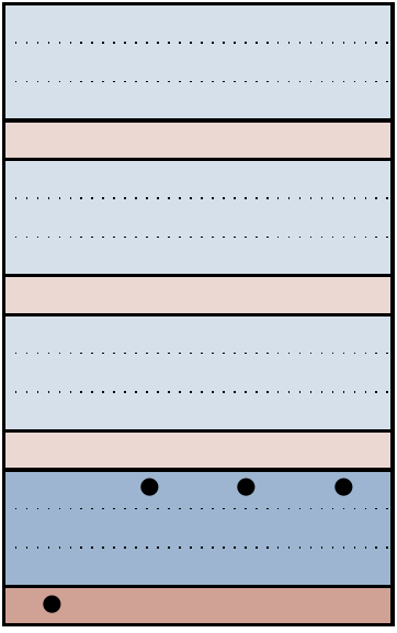
In the case of the three-qubit code, this corresponds to the possible physical errors being single phase-flips Z\mathbf{1}\mathbf{1}, \mathbf{1}Z\mathbf{1}, and \mathbf{1}\mathbf{1}Z. But here we see how misleading it is to omit mention of the identity error \mathbf{1}\mathbf{1}\mathbf{1}, because the single phase-flips all live in the same N(\mathcal{S}) coset as \mathbf{1}\mathbf{1}\mathbf{1}, but different \mathcal{S} cosets. That is, they are in the same error family, but a different row. By our above discussion, this means that we cannot correct for these errors — indeed, if we measure the error syndrome corresponding to “no error”, then we don’t know whether there truly was no error or if one of these single phase-flips happened instead. To put it succinctly, we nearly always make the assumption that no errors at all might occur, which is exactly the same as saying that the trivial error \mathbf{1} might occur. This means that we cannot correct for any errors that are found in the normaliser of \mathcal{S} but not in \mathcal{S} itself. Although this is technically a sub-rule of the previous rule, it’s worth pointing out explicitly.

An error-dot diagram describes a perfectly correctable set of errors if and only if the following two rules are satisfied:

1. In any given error family, all the dots are in the same row.
2. Any dots in the bottom error family are in the bottom row.

(The second rule follows from the first as long as the scenario in question allows the possibility for no errors to occur.)

Of course, we can state these conditions without making reference to the dot-error diagrams, instead using the same mathematical objects that we’ve been using all along. Proving the following version of the statement is the content of Exercise 14.11.12.

Let \mathcal{E}\subseteq\mathcal{P}_n be a set of physical errors. Then the stabiliser code defined by \mathcal{S} can perfectly correct for all errors in \mathcal{E} if and only if E_1^\dagger E_2 \in N(\mathcal{S})\setminus\mathcal{S} for all E_1,E_2\in\mathcal{E}.

You might notice that we’ve been sometimes been saying “perfectly correctable” instead of just “correctable”. This is because there might be scenarios where we are happy with being able to correct errors not perfectly, but instead merely with some high probability.

These dot-error diagrams are also able to describe more probabilistic scenarios. We have been saying “single-qubit errors”, but we could just have well have been saying “lowest-weight errors”, and then the assumption that errors are independent of one another means that higher-weight errors happen with lower probability. But the stabiliser formalism (and thus the error-dot diagrams) don’t care about this “independent errors” assumption! What this means is that we could refine our diagrams: instead of merely drawing dots to denote which errors can occur, we could also label them with specific probabilities. So we could describe a scenario where, for example, one specific high-weight error happens annoyingly often.

One last point that is important for those who care about mathematical correctness concerns our treatment of global phases.³⁰⁹ We do need to care about global phases in order to perform error-syndrome measurements, but once we have the error syndrome we can forget about them. In other words, we need the global phase in order to pick the error family, but not to pick a representative within it.

---

305. We will see these circuits soon, starting in Section 14.9.↩︎

306. Formally, we can think of ignoring phase as looking at the quotient of \mathcal{P}_3 by the subgroup \langle\pm\mathbf{1},\pm i\rangle, which results in an abelian group.↩︎

307. This is one of those arguments where it’s easy to get lost in the notation. Try picking two physical errors P_1 and P_2 in the same row somewhere in Figure 14.8 and following through the argument, figuring out what E, P, P'_1, and P'_2 are as you go.↩︎

308. Just to be clear, if we knew which physical errors took place, then we wouldn’t have to worry about error correction at all, because we’d always know how to perfectly recover the desired state. And remember that we can’t measure to find out which physical error took place, since this would destroy the state that we’re trying so hard to preserve!↩︎

309. We are being slightly informal with the way we draw these dot-error diagrams: cosets of \mathcal{S} itself inside \mathcal{P}_n don’t make sense, as we’ve said, because \mathcal{S} is generally not normal inside \mathcal{P}_n. Also, when we quotient by \{\pm1,\pm i\} (by drawing just a single sheet, instead of four as in the diagrams in Exercise 7.8.2), we make \mathcal{P} abelian, and this makes the normaliser no longer the actual normaliser.↩︎