14.10 Encoding arbitrary states

The encoding circuit in Figure 14.10 describes a unitary operation (it has no measurements), and its particularly compact form makes it very useful for certain complexity-theoretic calculations, but it has one major drawback: it is not itself protected against errors! If we are trying to design things for the real world, where qubits can undergo decoherence, then we should compensate for this in all our quantum computation, including the circuits we use to prepare states.³¹⁷ We have already done the hard work for this though, in Section 7.4, when we constructed circuits to project onto Pauli stabiliser spaces. This gives us the encoding circuit in Figure 14.11.

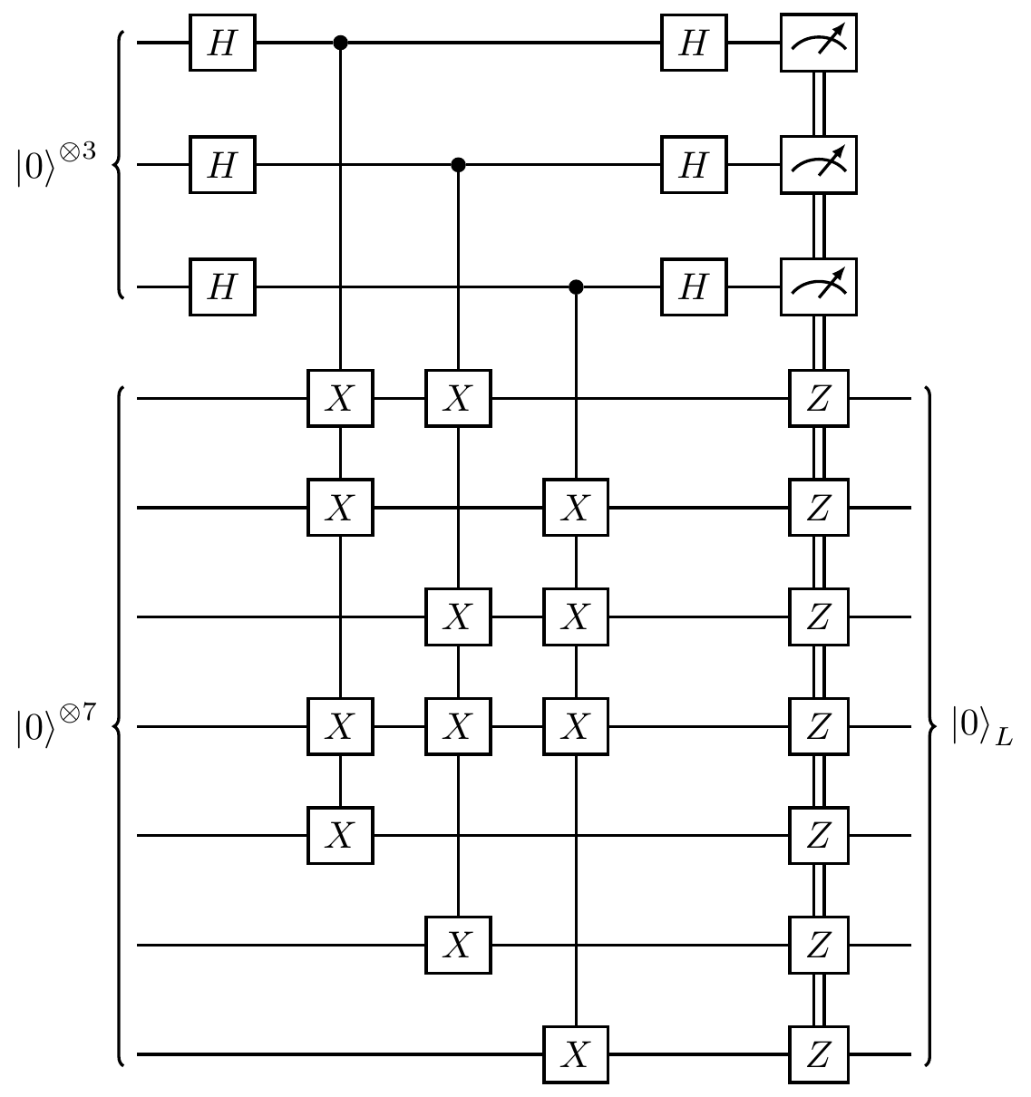
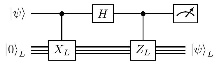
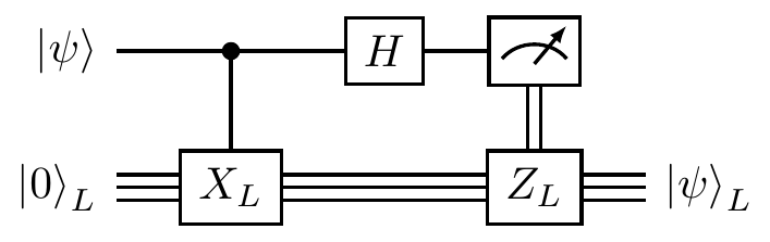
Figure 14.11: Another possible encoding circuit for the Steane code, which uses three ancilla bits for error correction when encoding arbitrary states, but is non-unitary (since it involves measurement). The measurements of the ancilla bits can be used to apply the necessary Z-type corrections.

The three measurements in the encoding circuit in Figure 14.11 allow us to correct for any single-qubit error in the encoding process, just as we did in Section 7.4, using the lookup table from Section 14.3. If we measure (+++), then no error has occurred, but if we measure, say, (-++), then we know that the error Z_5 has affected our encoding, and so we must correct for this. Of course, as we now know from Section 14.7, what it means to correct for the Z_5 error depends on which errors can possibly occur. If we make the usual assumption that only errors of weight 1 (i.e. single-qubit errors) can occur, then the Z_5 error is exactly that: a phase-flip on the fifth qubit.

So now we have seen two circuits for encoding the logical 0 state, but what about if we want to encode an arbitrary state? That is, we already have some qubit in an interesting state |\psi\rangle and we want to use the Steane code³¹⁸ to protect it against decoherence.

Before we look at this question, it’s important to mention something about practical use here. As is often the case, a chain is only as strong as its weakest link, and the process of encoding a single qubit into seven qubits is a particularly error-prone process. In practice, it is much more desirable to start with logical 0 and then do all of our computation, knowing that we are already in the “protected” world of a stabiliser code.

We know that all the X-type stabilisers for the Steane code have an even number of X terms in them, and so will commute with any implementation of the logical X operator X_L. Since the (bottom register of the) encoding circuit in Figure 14.11 simply applies the X-type stabilisers to |0\rangle^{\otimes7}, we can use this commutativity. Indeed, by construction of the logical operators and the logical states, we know that encoding |0\rangle^{\otimes7} to |0\rangle_L and then applying X_L gives us the state |1\rangle_L. But then the commutativity of X_L with the X-type stabilisers tells us that we also obtain |1\rangle_L if we first apply X_L to |0\rangle^{\otimes7} and then encode. Symbolically, writing E to mean the operation of applying the encoding circuit, \begin{aligned} |1\rangle_L &= X_L|0\rangle_L \\&= X_LE|0\rangle^{\otimes7} \\&= EX_L|0\rangle^{\otimes7} \end{aligned} where we can pick any implementation of X_L that we like, such as X^{\otimes7} or \mathbf{1}\mathbf{1}X\mathbf{1}\mathbf{1}XX. This tells us that there are two ways of obtaining |1\rangle_L from |0\rangle_L:

1. apply X_L and then encode
2. encode and then apply X_L.

Now let’s generalise this, replacing the X_L with a controlled version, controlled exactly by the state |\psi\rangle that we wish to encode. If |\psi\rangle=\alpha|0\rangle+\beta|1\rangle, then we want to construct the logical state |\psi\rangle_L \coloneqq \alpha|0\rangle_L + \beta|1\rangle_L. Let’s look at the first option from above: applying X_L and then encoding. For a simpler circuit, we can use the low-weight implementation \mathbf{1}\mathbf{1}X\mathbf{1}\mathbf{1}XX of X_L, so that we prepare the state \alpha|0\rangle_L + \beta|1\rangle_L = \alpha|0000000\rangle + \beta|0010011\rangle and then feed this into the encoding circuit from before. This gives us the circuit in Figure 14.12.

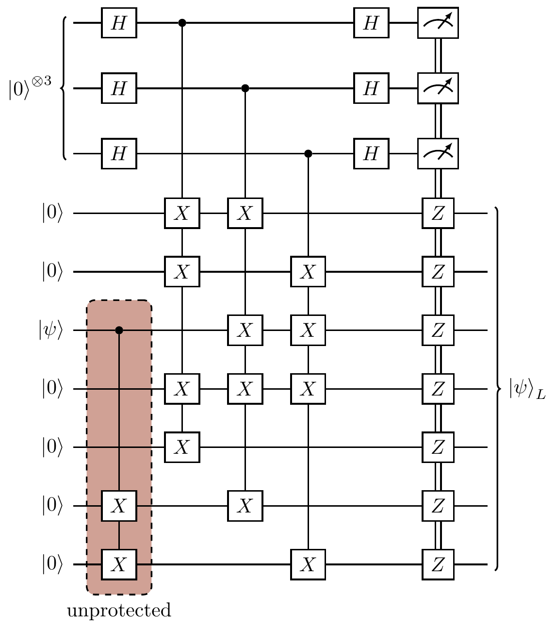
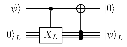
Figure 14.12: Preparing the logical version |\psi\rangle_L of an arbitrary state |\psi\rangle in a way that allows us to correct for any single-qubit errors in the encoding process, but not the preparation process (highlighted in red).

To repeat ourselves, the very first step of this circuit that enacts |0\rangle|0\rangle|\psi\rangle|0\rangle|0\rangle|0\rangle|0\rangle \longmapsto \alpha|0000000\rangle + \beta|0010011\rangle (where |\psi\rangle=\alpha|0\rangle + \beta|1\rangle) is not protected by any error correction scheme. If |\psi\rangle is some easily reproducible state, like |0\rangle, then we don’t really mind so much, since we could instead use a circuit where all seven qubits are initially in state |\psi\rangle, avoiding this problem altogether.³¹⁹ But if |\psi\rangle is the outcome of some previous computation, or just a state that we don’t have complete knowledge of, then we will always be faced with some uncertainty — did this preparation part of the circuit undergo an error or not? These sorts of problems are avoided if we can design truly fault-tolerant computational systems, instead of relying on mere error correction.

Now let’s look at the second option from before: encoding and then applying X_L. Imagine that we were able to construct the following circuit:

This would transfer the state |\psi\rangle=\alpha|0\rangle+\beta|1\rangle into a logical version |\psi\rangle_L, since it enacts the transformations \begin{aligned} (\alpha|0\rangle + \beta|1\rangle)|0\rangle_L &\longmapsto \alpha|0\rangle|0\rangle_L + \beta|1\rangle|1\rangle_L \\&\longmapsto |0\rangle(\alpha|0\rangle_L + \beta|1\rangle_L). \end{aligned} But what do we actually mean by this circuit? We haven’t defined controlled-X_L, nor what it means for a c-\texttt{NOT} to be controlled by a logical state.

The first is reasonably simple: if the control qubit is in state |1\rangle, then we want to apply X_L to the target. Since X_L can be³²⁰ expressed as a tensor product of Pauli X operators, this means that the controlled-X_L is just a bunch of controlled-\texttt{NOT} gates, each controlled by the top qubit, and targeting each of the qubits of the encoded state.

The second step is maybe not so obvious, but there’s a trick that we can use here! We know that the top qubit should end in the |0\rangle state, so we can do anything we want to it. For example, let’s apply a Hadamard gate and then measure it — why not?

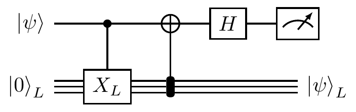
But now we can recall how controlled-\texttt{NOT} (which is simply a controlled-X) interacts with the Hadamard: the circuit above is equivalent to the circuit below.

This is a circuit that we could build, since we know all about the many implementations of X_L and Z_L thanks to the stabiliser formalism. If we really like, however, we could go one step further and replace the controlled-Z_L with a Z_L after the measurement:

---

317. If you want people to be able to stay dry if it’s raining, then you might build a tunnel from location A to location B so that they can use this for cover. But this isn’t going to stop people from getting wet on their (necessary) journey from their home to location A!↩︎

318. What we say here can be applied to other stabiliser codes, but we stick with the Steane code to make it easier to look at specific examples.↩︎

319. Thanks to the no-cloning theorem (Section 5.9), we know that there is no way of getting around this problem of only having one copy of the state |\psi\rangle that will work for any possible input — only if |\psi\rangle is something already known. So the preparation part of the circuit doesn’t clone the input state, but instead “smears it out” across three qubits instead of one, just like we mentioned in Section 13.7.↩︎

320. If we want to keep the circuit as simple as possible, then we should choose the smallest weight representative of X_L, which might not be just a tensor product of all X operators. For example, in the seven-qubit code there is an implementation of X_L of weight 3.↩︎