Remarks and exercises
Why qubits, subsystems, and entanglement?
One question that is rather natural to ask at this point is the following:
If entanglement is so fragile and difficult to control, then why bother?
Why not perform your computations in one singly physical system that has as many quantum states as we normally have labels for the states of qubits?
Then we could label these quantum states in the same way as we normally label the qubits, and give them computational meaning.
This suggestion, although possible, gives a very inefficient way of representing data, known as the unary encoding.
For serious computations, we need subsystems.
Here is why.
Suppose you have n physical objects, and each object has k distinguishable states.
If you can access each object separately and put it into any of the k states, then, with only n operations, you can prepare any of the k^{n} different configurations of the combined systems.
Without any loss of generality, let us take k=2 and refer to each object of this type as a physical bit.
We label the two states of a physical bit as 0 and 1.
So any collection of n physical bits can be prepared in 2^{n} different configurations, which can be used to store up to 2^{n} numbers (or binary strings, or messages, or however you want to interpret these things).
In order to represent numbers from 0 to N-1 we just have to choose n such that 2^n\geqslant N.
Suppose the two states in the physical bit are separated by the energy difference \Delta_E>0, i.e. that it costs \Delta_E units of energy to switch a physical bit from one state to the other.
Then a preparation of any particular configuration will cost no more than E=n \Delta_E=(\log_2 N)\Delta_E units of energy.
In contrast, if we choose to encode N configurations into one chunk of matter, say, into the first N energy states of a single harmonic oscillator with the same energy separation \Delta_E between states, then, in the worst case (i.e. going from the ground state 0 to the most excited state N) one has to use E=N\Delta_E units of energy.
For large N this gives an exponential gap in the energy expenditure between the binary encoding using physical bits, and the unary encoding using energy levels of harmonic oscillators: (\log_2 N)\Delta_E vs N\Delta_E.
Of course, you might try to switch to a different choice of realisation for the unary encoding, such as a quantum system that has a finite spread in the energy spectrum.
For example, by operating on the energy states of the hydrogen atom, you can encode any number from 0 to N-1, and we are guaranteed not to spend more than E_{\mathrm{max}}= 13.6\,\mathrm{eV} (otherwise the atom is ionised).
The snag is that, in this case, some of the electronic states will be separated by an energy difference to the order of E_{\mathrm{max}}/N, and to drive the system selectively from one state to another one has to tune into the frequency E_{\mathrm{max}}/\hbar N, which requires a sufficiently long wave packet in order for the frequency to be well defined, and consequently the
interaction time is of order N(\hbar/E_{\mathrm{max}}).
That is, we spend less energy, but the trade off is that we have to spend more time.
It turns out that whichever way we try to represent the number N in the unary encoding (i.e. using N different states of a single chunk of matter), we end up depleting our physical resources (such as energy or time, or even space) at a much greater rate than in the case when we use subsystems.
This plausibility argument indicates that, for efficient processing of information, the system must be divided into subsystems — for example, into physical bits.
Entangled or not?
Let a joint state of \mathcal{A} and \mathcal{B} be written in a product basis as
|\psi\rangle = \sum_{i,j} c_{ij}|a_i\rangle\otimes|b_j\rangle.
Assume that \mathcal{H}_{\mathcal{A}} and \mathcal{H}_{\mathcal{B}} are of equal dimension.
Show that, if |\psi\rangle is a product state, then \det (c_{ij}) = 0.
Show that the converse (\det(c_{ij})=0\implies|\psi\rangle=|a\rangle|b\rangle) holds only for qubits. Explain why.
Deduce that the state
\frac{1}{2}\big(|00\rangle + |01\rangle + |10\rangle + (-1)^k|11\rangle\big)
is entangled for odd values of k and unentangled for even values of k. Express the latter case explicitly as a product state.
Instantaneous communication
There is a lot of interesting physics behind the innocuous-looking mathematical statement of Exercise 5.14.2.
For example, think again about the state (|00\rangle+|11\rangle)/\sqrt{2}.
What happens if you measure just the first qubit?
It is equally likely that you get |0\rangle or |1\rangle, right?
But after your measurement the two qubits are either in state |00\rangle or in |11\rangle, i.e. they show the same bit value.
Now, why might that be disturbing?
Well, imagine the second qubit to be light-years away from the first one.
It seems that the measurement of the first qubit affects the second qubit right away, which seems to imply faster-than-light communication!
This is what Einstein called “spooky action as a distance” in his 1947 letter to Max Born.
But can you actually use this effect to send a message faster than light?
What would happen if you tried?
Hopefully you can see that it would not work, since the result of the measurement is random: you cannot choose the bit value you want to send.
We shall return to this, and other related phenomena, later on — it is not at all a lost cause!
SWAP circuit
Show that, for any states |\psi_1\rangle and |\psi_2\rangle of two qubits, the circuit below implements the \texttt{SWAP} operation |\psi_1\rangle|\psi_2\rangle \mapsto |\psi_2\rangle|\psi_1\rangle.
Controlled-NOT circuit
Show that the circuit below gives another implementation of the controlled-\texttt{NOT} gate.
(Controlled-\texttt{NOT}, again).

Measuring with controlled-NOT
The controlled-\texttt{NOT} gate can act as a measurement gate: if you prepare the target in state |0\rangle then the gate acts as |x\rangle|0\rangle\mapsto|x\rangle|x\rangle, and so the target learns the bit value of the control qubit.
If you wish, you can think about a subsequent measurement of the target qubit in the computational basis as an observer learning about the bit value of the control qubit.
Take a look at the circuit below, where M stands for measurement in the standard basis.
Now assume that the top two qubits are in the state
|\psi\rangle
= \frac{1}{\sqrt3}\big( |01\rangle - |10\rangle + i|11\rangle \big).
The measurement M gives two possible outcomes: 0 and 1.
What are the probabilities of each outcome, and what is the post-measurement state in each case?
What is this circuit actually measuring?
Arbitrary controlled-U on two qubits
Recall Section 3.5: any unitary operation U on a single qubit can be expressed as
U = B^\dagger XBA^\dagger XA
for some unitaries A and B, where X\equiv\sigma_x is the Pauli bit-flip operator.
Suppose that you can implement any single-qubit gate, and that you have a bunch of controlled-\texttt{NOT} gates at your disposal.
How would you implement any controlled-U operation on two qubits?
Entangled qubits
Two entangled qubits in the state \frac{1}{\sqrt{2}}(|00\rangle+|11\rangle) are generated by some source S.
One qubit is sent to Alice, and one to Bob, who then both perform measurements in the computational basis.
What is the probability that Alice and Bob will register identical results?
Can any correlations they observe be used for instantaneous communication?
Prior to the measurements in the computational basis, Alice and Bob apply unitary operations R_\alpha and R_\beta (respectively), for some fixed values \alpha,\beta\in\mathbb{R}, to their respective qubits:
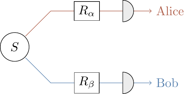
where the gate R_\theta is defined by its action on the basis states:
\begin{aligned}
|0\rangle
&\longmapsto
\cos\theta|0\rangle + \sin\theta|1\rangle
\\|1\rangle
&\longmapsto
-\sin\theta|0\rangle + \cos\theta|1\rangle.
\end{aligned}
Show that the state of the two qubits prior to the measurements is
\begin{aligned}
&\frac{1}{\sqrt{2}}\cos(\alpha-\beta)\big( |00\rangle + |11\rangle \big)
\\- &\frac{1}{\sqrt{2}}\sin(\alpha-\beta)\big( |01\rangle - |10\rangle \big).
\end{aligned}
What is the probability that Alice and Bob’s outcomes are identical?
What is the geometric interpretation of the operator R_\theta?
Playing with conditional unitaries
The swap gate \texttt{SWAP} on two qubits is defined first on product vectors by \texttt{SWAP}\colon|a\rangle|b\rangle\mapsto|b\rangle|a\rangle and then extended to sums of product vectors by linearity (see Exercise 5.14.4).
Show that the four Bell states \frac{1}{\sqrt{2}}(|00\rangle\pm|11\rangle) and \frac{1}{\sqrt{2}}(|01\rangle\pm|10\rangle) are eigenvectors of \texttt{SWAP} that form an orthonormal basis in the Hilbert space associated to two qubits.
Which Bell states span the symmetric subspace (i.e. the space spanned by all eigenvectors with eigenvalue 1), and which the antisymmetric one (i.e. that spanned by eigenvectors with eigenvalue -1)?
Can \texttt{SWAP} have any eigenvalues apart from \pm1?
Show that P_\pm = \frac{1}{2}(\mathbf{1}\pm \texttt{SWAP}) are two orthogonal projectors which form the decomposition of the identity and project onto the symmetric and antisymmetric subspaces.
Decompose the state vector |a\rangle|b\rangle of two qubits into symmetric and antisymmetric components.
Consider the quantum circuit below, composed of two Hadamard gates, one controlled-\texttt{SWAP} operation (also known as the controlled-swap, or Fredkin gate), and the measurement M in the computational basis.
Suppose that the state vectors |a\rangle and |b\rangle are normalised but not orthogonal to one another.
Step through the execution of this network, writing down the quantum states of the three qubits after each of the four computational steps.
What are the probabilities of observing 0 or 1 when the measurement M is finally performed?
(Symmetric and antisymmetric projection).

Explain why this quantum network implements projections on the symmetric and antisymmetric subspaces of the two qubits.
Two qubits are transmitted through a quantum channel which applies the same randomly chosen unitary operation U to each of them, i.e. U\otimes U.
Show that the symmetric and antisymmetric subspaces are invariant under this operation.
Polarised photons are transmitted through an optical fibre.
Due to the variation of the refractive index along the fibre, the polarisation of each photon is rotated by the same unknown angle.
This makes communication based on polarisation encoding unreliable.
However, if you are able to prepare any polarisation state of the two photons then you can still use the channel to communicate without any errors — how?
Tensor products in components
In our discussion of tensor products we have so far taken a rather abstract approach.
There are, however, situations in which we have to put numbers in, and write tensor products of vectors and matrices explicitly.
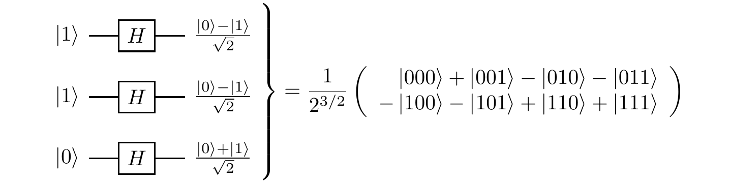
For example, here is the standard basis of two qubits written explicitly as column vectors:
\begin{aligned}
|00\rangle &\equiv |0\rangle\otimes|0\rangle
= \begin{bmatrix}1\\0\end{bmatrix} \otimes \begin{bmatrix}1\\0\end{bmatrix}
= \begin{bmatrix}1\\0\\0\\0\end{bmatrix}
\\[1em]
|01\rangle &\equiv |0\rangle\otimes|1\rangle
= \begin{bmatrix}1\\0\end{bmatrix} \otimes \begin{bmatrix}0\\1\end{bmatrix}
= \begin{bmatrix}0\\1\\0\\0\end{bmatrix}
\\[1em]
|10\rangle &\equiv |1\rangle\otimes|0\rangle
= \begin{bmatrix}0\\1\end{bmatrix} \otimes \begin{bmatrix}1\\0\end{bmatrix}
= \begin{bmatrix}0\\0\\1\\0\end{bmatrix}
\\[1em]
|11\rangle &\equiv |1\rangle\otimes|1\rangle
= \begin{bmatrix}0\\1\end{bmatrix} \otimes \begin{bmatrix}0\\1\end{bmatrix}
= \begin{bmatrix}0\\0\\0\\1\end{bmatrix}
\end{aligned}
Given |a\rangle = \alpha_0|0\rangle + \alpha_1|1\rangle and |b\rangle = \beta_0|0\rangle +\beta_1|1\rangle, we write |a\rangle\otimes|b\rangle as
\begin{aligned}
|a\rangle\otimes|b\rangle
&= \begin{bmatrix}\alpha_0\\\alpha_1\end{bmatrix} \otimes \begin{bmatrix}\beta_0\\\beta_1\end{bmatrix}
\\&= \begin{bmatrix}\alpha_0\begin{bmatrix}\beta_0\\\beta_1\end{bmatrix}\\\alpha_1\begin{bmatrix}\beta_0\\\beta_1\end{bmatrix}\end{bmatrix}
\\&= \begin{bmatrix}\alpha_0\beta_0\\\alpha_0\beta_1\\\alpha_1\beta_0\\\alpha_1\beta_1\end{bmatrix}.
\end{aligned}
Note that each element of the first vector multiplies the entire second vector.
This is often the easiest way to get the tensor products in practice.
The matrix elements of the tensor product operation A\otimes B

are given by
(A\otimes B)_{ik,jl} = A_{ij}B_{kl}
where ik\in\{00,01,10,11\} labels the rows, and kl\in\{00,01,10,11\} labels columns, when forming the block matrix:
\begin{aligned}
A\otimes B
&= \begin{bmatrix}A_{00}&A_{01}\\A_{10}&A_{11}\end{bmatrix} \otimes \begin{bmatrix}B_{00}&B_{01}\\B_{10}&B_{11}\end{bmatrix}
\\&= \begin{bmatrix}A_{00}B&A_{01}B\\A_{10}B&A_{11}B\end{bmatrix}
\\&=
\left[
\,
\begin{array}{c|c}
\begin{matrix}A_{00}B_{00}&A_{00}B_{01}\\A_{00}B_{10}&A_{00}B_{11}\end{matrix}
& \begin{matrix}A_{01}B_{00}&A_{01}B_{01}\\A_{01}B_{10}&A_{01}B_{11}\end{matrix}
\\\hline
\begin{matrix}A_{10}B_{00}&A_{10}B_{01}\\A_{10}B_{10}&A_{10}B_{11}\end{matrix}
& \begin{matrix}A_{11}B_{00}&A_{11}B_{01}\\A_{11}B_{10}&A_{11}B_{11}\end{matrix}
\end{array}
\,
\right]
\end{aligned}
The tensor product induces a natural partition of matrices into blocks.
Multiplication of block matrices works pretty much the same as regular matrix multiplication (assuming the dimensions of the sub-matrices are appropriate), except that the entries are now matrices rather than numbers, and so may not commute.
Evaluate the following matrix product of (4\times 4) block matrices:
\left[
\,
\begin{array}{c|c}
\mathbf{1}& X
\\\hline
Y & Z
\end{array}
\,
\right]
\left[
\,
\begin{array}{c|c}
\mathbf{1}& Y
\\\hline
X & Z
\end{array}
\,
\right]
(where X, Y, and Z are the Pauli matrices).
Using the block matrix form of A\otimes B expressed in terms of A_{ij} and B_{ij} (as described above), explain how the following operations are performed on the block matrix:
- transposition (A\otimes B)^T;
- partial transpositions A^T\otimes B and A\otimes B^T;
- trace \operatorname{tr}(A\otimes B);
- partial traces (\operatorname{tr}A)\otimes B and A\otimes(\operatorname{tr}B).
The Schmidt decomposition
An arbitrary vector in the Hilbert space \mathcal{H}_{\mathcal{A}}\otimes \mathcal{H}_{\mathcal{B}} can be expanded in a product basis as
|\psi\rangle
= \sum_{i,j} c_{ij}|a_i\rangle|b_j\rangle.
Moreover, for any given joint state |\psi\rangle, we can find orthonormal bases, \{|\tilde{a}_i\rangle\} in \mathcal{H}_{\mathcal{A}} and \{|\tilde{b}_j\rangle\} in \mathcal{H}_{\mathcal{B}}, such that |\psi\rangle can be expressed as
|\psi\rangle
= \sum_{i} d_{i}|\tilde a_i\rangle|\tilde b_i\rangle,
where the coefficients d_i are non-negative numbers.
This is known as the Schmidt decomposition of |\psi\rangle.
Any bipartite state can be expressed in this form, but remember that the bases used depend on the state being expanded.
Indeed, given two bipartite states |\psi\rangle and |\phi\rangle, we usually cannot perform the Schmidt decomposition using the same orthonormal bases in \mathcal{H}_{\mathcal{A}} and \mathcal{H}_{\mathcal{B}}.
The number of terms in the Schmidt decomposition is, at most, the minimum of \dim\mathcal{H}_{\mathcal{A}} and \dim\mathcal{H}_{\mathcal{B}}.
The Schmidt decomposition follows from the singular value decomposition (often abbreviated to SVD): any (n\times m) matrix C can be written as
C = UDV
where U and V are (respectively) (n\times n) and (m\times m) unitary matrices, and D is an (n\times m) diagonal matrix with real, non-negative elements in descending order d_1\geqslant d_2\geqslant\ldots\geqslant d_{\min\{n,m\}} (and with the rest of the matrix is filled with zeros).
The elements d_k are called the singular values of C.
We will return to the SVD in more detail later on, in Section 12.11.1.
You can visualize the SVD by thinking of C as representing a linear
transformation from m-dimensional to n-dimensional Euclidean space: it maps the unit ball in the m-dimensional space to an ellipsoid in
the n-dimensional space; the singular values are the lengths of
the semi-axes of that ellipsoid; the matrices U and V carry
information about the locations of those axes and the vectors in
the first space which map into them.
Thus SVD tells us that the transformation C consists of rotating the unit ball (the transformation V), stretching the k-th axis by a factor of d_k (the transformation D), and then rotating the resulting ellipsoid (the transformation U).
Using the index notation C_{ij} = \sum_k U_{ik}d_k V_{kj}, we can thus apply SVD to c_{ij}:
\begin{aligned}
|\psi\rangle
&= \sum_{i,j} c_{ij}|a_ib_j\rangle
\\&= \sum_{i,j} \sum_k U_{ik}d_k V_{kj}|a_ib_j\rangle
\\&= \sum_k d_k \left(\sum_i U_{ik}|a_i\rangle\right)\otimes\left(\sum_j V_{kj}|b_j\rangle\right).
\end{aligned}
The Schmidt decomposition of a separable state of the form
|a\rangle\otimes|b\rangle is trivially just this state.
The Bell states \Psi^+ and \Phi^+ are already written in their Schmidt form, whereas \Psi^- and \Phi^- can be easily expressed in the Schmidt form.
For example, for |\Psi^-\rangle we have d_1 = d_2 = \frac{1}{\sqrt{2}}, and the Schmidt basis is
\begin{aligned}
|\tilde{a}_1\rangle &= |0\rangle
\\|\tilde{a}_2\rangle &= |1\rangle
\\|\tilde{b}_1\rangle &= |1\rangle
\\|\tilde{b}_2\rangle &= -|0\rangle.
\end{aligned}
The number of non-zero singular values of c_{ij} is called the rank of c_{ij}, or the rank of the corresponding quantum state, or sometimes, the Schmidt number.
You should be able to see that all bipartite states of rank-one are separable.
The Schmidt decomposition is almost unique.
The ambiguity arises when we have two or more identical singular values, as, for example, in the case of the Bell states.
Then any unitary transformation of the basis vectors corresponding to a degenerate singular value, both in \mathcal{H}_a and in \mathcal{H}_b, generates another set of basis vectors.