1.6 Qubits, gates, and circuits
Atoms, trapped ions, molecules, nuclear spins, and many other quantum objects with two pre-selected basis states labelled as
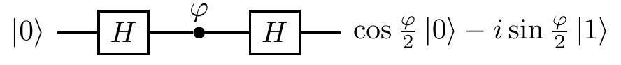
This diagram should be read from left to right. The horizontal line represents a qubit that is inertly carried from one quantum operation to another. We often call this line a quantum wire. The wire may describe translation in space (e.g. atoms travelling through cavities) or translation in time (e.g. a sequence of operations performed on a trapped ion).32 The boxes or circles on the wire represent elementary quantum operations, called quantum (logic) gates.
In the example circuit above, we have two types of gates: two Hadamard gates
The input qubits appear as state vectors on the left side of circuit diagrams, and the output qubits as state vectors on the right.
The product of the three matrices34
Do not confuse the interference diagrams of Figure 1.1 and Figure 1.3 with the circuit diagram. In the circuit diagrams, which we will use almost constantly from now on, a single line represents a single qubit.↩︎
Yet again we see that we can conveniently forget about the actual physical implementations, treating them all with the same abstract description.↩︎
Global phase factors are irrelevant; it is only the relative phase
\varphi =\varphi_1-\varphi_0 that matters. For example, in a single-qubit phase gateP_\varphi we usually factor oute^{i\varphi_0} , leaving us with the two diagonal entries:1 ande^{i\varphi} .↩︎cf. Figure 1.3. Note again that circuits are read left to right, but matrix composition goes right to left. Since the first and last matrices/gates are the same (i.e. both are
H ), we don’t notice this, but it’s important to note that the first (i.e. leftmost)H in the matrix productHP_\varphi H corresponds to the last (i.e. rightmost)H in the circuit diagram.↩︎