How far apart are two probability distributions?
Before we switch gears and discuss how to generalise state distance to density operators, let us first take a look at distances between probability distributions.
What does it mean to say that two probability distributions (over the same index set) are similar to one another?
Recall that a probability distribution consists of two things — a sample space \Omega, which is the set of all possible outcomes, and a probability function p\colon\Omega\to[0,1], which tells us the probability of any specific outcome — subject to the condition that \sum_{k\in\Omega} p(k)=1.
Given any subset of outcomes A\subseteq\Omega, we define p(A)=\sum\{k\in A\}p(k).
The trace distance (also known as the variation distance, L_1 distance, statistical distance, or Kolmogorov distance) between probability distributions p and q on the same sample space \Omega is
d(p,q) \coloneqq \frac{1}{2}\sum_{k\in\Omega} |p(k)-q(k)|.
This is indeed a distance: it satisfies all the necessary properties.
It also has a rather simple interpretation, as we now explain.
Let p(k) be the intended probability distribution of an outcome produced by some ideal device P, but suppose that the actual physical device Q is slightly faulty: with probability 1-\varepsilon it works exactly as P does, but with probability \varepsilon it goes completely wrong and generates an output according to some arbitrary probability distribution e(k).
What can we say about the probability distribution q(k) of the outcome of such a device?
Well, we can exactly say that
d(p,q) \leqslant\varepsilon
by substituting q(k)=(1-\varepsilon)p(k)+\varepsilon e(k).
Conversely, if d(p,q)=\varepsilon then we can represent one of them (say, q(k)) as the probability distribution resulting from a process that generates outcomes according to p(k) followed by a process that alters outcome k with total probability not greater than \varepsilon.
Note that the normalisation property of probabilities implies that
\sum_k p(k)-q(k) = 0.
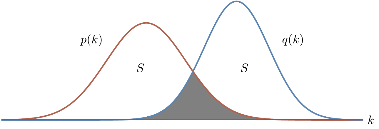
We can split up this sum into two parts: the sum over k for which p(k)\geqslant q(k), and the sum over k for which p(k)<q(k).
If we call the first part S, then the fact that \sum_k p(k)-q(k)=0 tells us that the second part must be equal to -S.
Thus
\sum_k |p(k)-q(k)|
= S+|-S|
= 2S
whence S=d(p,q).
Just as a passing note, we will point out that
\begin{aligned}
\sum_k \max\{p(k),q(k)\}
&= 1 + S
\\&= 1 + d(p,q)
\end{aligned}
and the shaded area in Figure 12.1 is equal to
\begin{aligned}
\sum_k \min\{p(k),q(k)\}
&= 1 - S
\\&= 1 - d(p,q).
\end{aligned}
The latter lets us write the trace distance as
d(p,q) = 1 - \sum_k \min_k\{p(k),q(k)\}
and the former will be useful very soon.
As for intuition, the trace distance is a measure of how well we can distinguish a sample from distribution p from a sample from distribution q: if the distance is 1 then we can tell them apart perfectly; if the distance is 0 then we can’t distinguish them at all.
Now suppose that p and q represent the probability distributions of two devices, P and Q, respectively, and that one of these is chosen (with equal probability) to generate some outcome.
If you are given the outcome k, and you know p(k) and q(k), then how can you best guess which device generated it?
What is your best strategy, and with what probability does this let you guess correctly?
It turns out that we can answer this using the trace distance.
Arguably the most natural strategy is to look at \max\{p(k),q(k)\}: guess P if p(k)>q(k); guess Q if q(k)>p(k); guess uniformly at random if p(k)=q(k).
Following this strategy, the probability of guessing correctly (again, under the assumption that P and Q were chosen between with equal probability) is
p_{\mathrm{success}} = \frac{1}{2}\sum_k \max\{p(k),q(k)\}
which we can rewrite as
p_{\mathrm{success}} = \frac{1}{2}(1+d(p,q)).
Here is another way of seeing the above.
The probability that the devices P and Q will not behave in the same way is bounded by d(p,q).
This means that, with probability 1-d(p,q), the devices behave as if they were identical, in which case the best you can do is to guess uniformly at random, which will make you succeed with probability \frac{1}{2}(1-d(p,q)).
With the remaining probability d(p,q), the devices may behave as if they were completely different, and then you can tell which one is which perfectly, letting you succeed with probability exactly 1\cdot d(p,q)=d(p,q).
So the total probability of success is equal to
\frac{1}{2}(1-d(p,q)) + d(p,q)
= \frac{1}{2}(1+d(p,q)).