14.1 The Hamming code

The challenge in designing efficient error-correcting codes resides in the trade-off between rate and distance (introduced in Section 13.6). Ideally, both quantities should be high: a high rate signifies low overhead in the encoding process (i.e. requiring only a few redundant bits), and a high distance means that many errors can be corrected. So can we optimise both of these quantities simultaneously? Unfortunately, various established bounds tell us that there is always a trade off, so high-rate codes must have low distance, and high-distance codes must have a low rate. Still, there is a lot of ingenuity that goes into designing good error-correction codes, and some are still better than others!

Before looking at quantum codes in more depth, we again start with classical codes. For example, in Section 13.6 we saw the three-bit repetition code, which has a rate of R=1/3 and distance 3. However, the Hamming [7,4,3] code²⁷⁹ has the same distance, but a better rate of R=4/7>1/3. Figure 14.1 show diagrammatic representations of this Hamming code, which we will now study further.

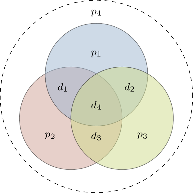
Figure 14.1: Left: The Venn diagram for the Hamming [7,4,3] code. Right: The plaquette (or finite projective plane) diagram for the same code. In both, d_i are the data bits and the p_i are the parity bits. The coloured circles (resp. coloured quadrilaterals) are called plaquettes.

We say that the plaquette diagram in Figure 14.1 could also be called a finite projective plane diagram because of how it resembles the Fano plane, which is the projective space of dimension 2 over the field with 2 elements.

In fact, there is more than a mere visual similarity between these two diagrams: we will soon introduce the formal definition of a linear code, and there is a special family of these known as projective codes, which are those such that the columns of the generator matrix (another character who we shall soon meet) are all distinct and non-zero.

Projective codes are particularly interesting because they allow us to apply geometric methods to study the properties of the code. For example, the columns of the parity check matrix of a projective code correspond to points in some projective space. Furthermore, since the geometry in question concerns finite dimensional spaces over finite fields, we end up coming across a lot of familiar (and useful) combinatorics. This is partially due to the fact that finite geometry can be understood as an example of an incidence structure.

Both diagrams in Figure 14.1 describe the same situation, but although the right-hand one is useful for understanding the geometry hidden in the construction and allowing us to generalise to create new codes, and is thus the one that we will tend to use, the Venn diagram on the left-hand side is maybe more suggestive of what’s going on.

The idea is that we have a four-bit string d_1d_2d_3d_4 consisting of the four data bits, and we encode into a seven-bit string²⁸⁰ d_1d_2d_3d_4p_1p_2p_3 by appending three parity bits p_1, p_2, and p_3, which are defined by \begin{aligned} p_1 &= d_1 + d_2 + d_4 \ \mathrm{mod}\ 2 \\p_2 &= d_1 + d_3 + d_4 \ \mathrm{mod}\ 2 \\p_3 &= d_2 + d_3 + d_4 \ \mathrm{mod}\ 2. \end{aligned} You can hopefully see how the triangular diagram in Figure 14.1 tells us which data bits are used in defining each parity bit: we take the sum of all data bits in the same plaquette (one of the three coloured quadrilaterals) as the parity bit.

We can also express this encoding in matrix notation, defining the data vector \mathbf{d} by \mathbf{d} = \begin{bmatrix} d_1\\d_2\\d_3\\d_4 \end{bmatrix} and the generator matrix²⁸¹ G by G = \begin{bmatrix} \begin{array}{cccc} 1 & 0 & 0 & 0 \\0 & 1 & 0 & 0 \\0 & 0 & 1 & 0 \\0 & 0 & 0 & 1 \\\hline 1 & 1 & 0 & 1 \\1 & 0 & 1 & 1 \\0 & 1 & 1 & 1 \end{array} \end{bmatrix}

The vector space spanned by the columns of the generator matrix G is known as the codespace of the code, and any vector in this space is known as a codeword.

The encoding process is then given by the matrix G acting on the vector \mathbf{d}. Indeed, since the top (4\times4) part of G is the identity, the first four rows of the output vector G\mathbf{d} will simply be a copy of \mathbf{d}; the bottom (3\times4) part of G is chosen precisely so that the last three rows of G\mathbf{d} will be exactly p_1, p_2, and p_3. In other words, G\mathbf{d} = \begin{bmatrix} d_1\\d_2\\d_3\\d_4\\p_1\\p_2\\p_3 \end{bmatrix} = \begin{bmatrix} \mathbf{d}\\p_1\\p_2\\p_3 \end{bmatrix}.

By construction, the sum of the four bits in any single plaquette of the code sum to zero.²⁸² For example, in the bottom-left (red) plaquette, \begin{aligned} p_2 + d_1 + d_3 + d_4 &= d_1 + d_3 + d_4 + d_1 + d_3 + d_4 \\&= 2(d_1 + d_3 + d_4) \\&= 0 \end{aligned} and the same argument holds for the other two plaquettes. This incredibly simple fact is where the power of the Hamming code lies, since it tells the receiver of the encoded string a lot of information about potential errors.

Let’s consider a concrete example. Say that Alice encodes her data string d_1d_2d_3d_4 and sends the result G\mathbf{d} to Bob, who takes this vector and looks at the sum of the bits in each plaquette, and obtains the following:²⁸³

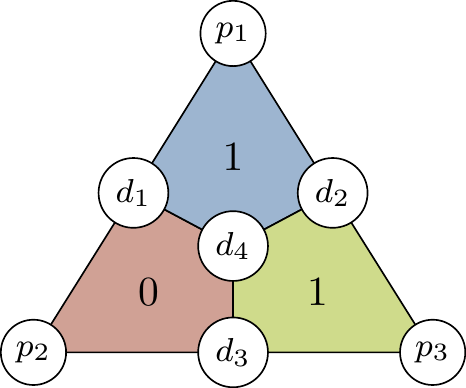
If we make the assumption that at most one error occurs²⁸⁴ then this result tells us exactly where the bit-flip happened: it is not in the bottom-left (red) plaquette, but it is in both the top (blue) and bottom-right (yellow) plaquettes. Looking at the diagram we see that it must be d_2 that was flipped, and so we can correct for this error by simply flipping it back before unencoding (where the unencoding process is given by simply forgetting the last three bits of the received string).

We can describe the error location process in terms of matrices as well, using the parity-check matrix²⁸⁵ H, given by H = \begin{bmatrix} \begin{array}{cccc|ccc} 1 & 1 & 0 & 1 & 1 & 0 & 0 \\1 & 0 & 1 & 1 & 0 & 1 & 0 \\0 & 1 & 1 & 1 & 0 & 0 & 1 \end{array} \end{bmatrix}. Note that the rows of H are exactly the coefficients of the parity-check equations for each plaquette, where we order them top–left–right (blue–red–yellow). For example, to get the sum corresponding to the bottom-left (red) plaquette, we need to sum the first, third, fourth, and sixth bits of the encoded string d_1d_2d_3d_4p_1p_2p_3, and these are exactly the non-zero entries of the second row of H. The columns of the parity-check matrix H are known as the error syndromes, for reasons we will now explain

The parity-check matrix H is defined exactly so that²⁸⁶ H\mathbf{c} = 0 \iff \mathbf{c}\text{ is a codeword}. Now we can see a bit more into how things work, since linearity of matrix multiplication tells us that, if a receiver receives \mathbf{c}+\mathbf{e} where \mathbf{e} is the error, \begin{aligned} H(\mathbf{c}+\mathbf{e}) &= H\mathbf{c}+H\mathbf{e} \\&=H\mathbf{e}. \end{aligned} Decoding the message then consists of finding the most probable error \mathbf{e} that yields the output H\mathbf{e}. If \mathbf{e} is a single bit-flip error, then H\mathbf{e} is exactly a column of H, which justifies us describing the columns as error syndromes. We can construct a table describing all of the possible error syndromes, and which bit they indicate for us to correct:

Syndrome	000	110	101	011	111	100	010	001
Correction	-	d_1	d_2	d_3	d_4	p_1	p_2	p_3

The above construction of the Hamming [7,4,3] code can be generalised to result in a Hamming [2^r-1,2^r-r-1,3] code²⁸⁷ for any r\geqslant 2, where each column of the parity-check matrix is a different binary string, excluding the string of all 0 bits. It’s noteworthy that only a logarithmic number of parity checks are necessary to correct all single-bit errors. However, there are some downsides to Hamming codes. Although the rate R=(2^r-r-1)/(2^r-1) approaches 1 as r\to\infty, Hamming codes are impractical in highly noisy environments because they have a fixed distance of 3.

Although the Hamming [7,4,3] code can only deal with single-bit errors, it can be extended to an [8,4,4] code, at least detecting double-bit errors, by adding a single extra parity bit p_4, given by taking the sum of all the other seven bits:

How does this work? Well, let’s assume that up to two bit-flip errors could occur. The decoding process then starts by looking at this new parity bit p_4 in the received string and seeing if it is indeed equal to the sum of all the other bits, saying that it is “correct” if so, and “incorrect” if not. If p_4 is incorrect, then there has been a single-bit error, and we can just look at the rest of the string d_1d_2d_3d_4p_1p_2p_3 and apply the previous Hamming [7,4,3] code decoding process, with the caveat that if this tells us that no errors have occurred, then it must be the case that the single-bit error actually flipped the parity bit p_4 itself. If p_4 is correct, then there has either been no error or a double bit-flip error; to see which is the case we can measure the Hamming [7,4,3] code error syndrome of d_1d_2d_3d_4p_1p_2p_3, and this will tell us the \texttt{XOR} of the two bit-flip locations; if this is 0 then either no error has occurred or two errors affected the same bit, cancelling each other out.

Before moving on, it will be useful to introduce another common way of diagrammatically representing parity-check matrices called a Tanner graph. This is a bipartite graph²⁸⁸ consisting of two types of nodes: the codeword (or data) nodes (one for each bit of the codeword, drawn as circles), and the syndrome nodes (one for each bit of the syndrome, drawn as squares). The edges in the Tanner graph are such that the parity-check matrix H is exactly the adjacency matrix of the graph, i.e. the matrix that has a 1 in the (i,j)-th position if the i-th syndrome node is connected to the j-th codeword node, and a 0 otherwise.

Figure 14.2: The Tanner graph for the Hamming [7,4,3] code. Comparing this to the plaquette diagram in Figure 14.1, we see that we simply replace plaquettes by syndrome nodes (hence our choice of colours). It is not immediately evident that this graph is bipartite, but try drawing it with all the syndrome nodes in one row and all the data nodes in another row below to see that it is.

One particularly useful aspect of Tanner graphs is how simple it is to convert to and from the corresponding parity-check quantum circuits. There is a syndrome node for each ancilla qubit, and a data node for each data qubit; there are paths between syndrome and data nodes whenever there is a controlled-\texttt{NOT} between the corresponding qubits. We show a simple example in Figure 14.3.

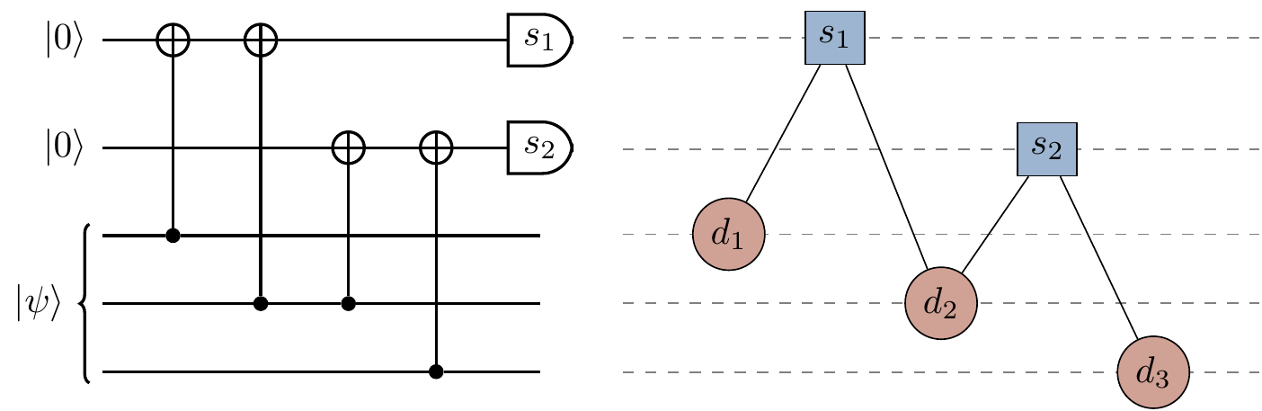
Figure 14.3: Left: The quantum circuit for a parity-check operation. Right: The corresponding Tanner graph.

---

279. In the late 1940s, Richard Hamming, working at Bell Labs, was exasperated by the fact that the machines running his punch cards (in these heroic times of computer science, punch cards were the state of the art data storage) were good enough to notice when there was an error (and halting) but not good enough to know how to fix it.↩︎

280. Sometimes you will see the Hamming [7,4,3] code referred to simply as the seven-bit Hamming code, the [7,4,3] code, or even just the Hamming code.↩︎

281. Many sources define G to be the transpose of what we use here, but this is just a question of convention. Because of this, we’ll be dealing with the column (not row) spaces of matrices, also known as the range.↩︎

282. Since we are working with classical bits, all addition is taken \ \mathrm{mod}\ 2, so sometimes we will neglect to say this explicitly.↩︎

283. We don’t write the values of the bits, only the sums of the bits in each plaquette. This is because we don’t need to know the value of the bits in order to know where the error is, only the three sums!↩︎

284. This assumption is crucial here, and we investigate what happens if we drop it in Section 14.7.↩︎

285. Here is yet another H, to go with the Hadamard and the Hamiltonian…↩︎

286. Recall that codewords are exactly those vectors of the form G\mathbf{d} for some data vector \mathbf{d}↩︎

287. How do we know that the distance is always 3? Well, there are triples of columns in the parity-check matrix that, when added together, give all zeros. This means that there are sets of 3 errors such that, if they all occur together, the syndrome will be zero, and so the distance is no more than 3. Meanwhile, all the columns are distinct, so no pair of columns add together trivially, which means that the distance must be greater than 2.↩︎

288. A graph (which is a collection of nodes and edges between some of them) is bipartite if the nodes can be split into two sets such that all the edges go from one element of the first set to one element of the second.↩︎