Correcting bit-flips
In order to protect a qubit against bit-flips (thought of as incoherent X rotations), we rely on the same classical repetition code as in Section 13.6, but both encoding and error correction are now implemented by quantum operations.
Let’s return to the example of the three-qubit code that we introduced in Section 13.1.
We take a qubit in some unknown pure state \alpha|0\rangle+\beta|1\rangle and encode it into three qubits, introducing two auxiliary qubits:
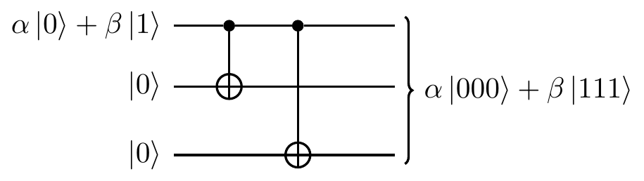
Mathematically, this is an isometric embedding of a two-dimensional space into an eight-dimensional one.
It is important to note that this is not just the classical repetition code “but with qubits instead of bits” — this would be impossible to construct, since the no-cloning theorem tells us that we can never build a circuit that enacts
\alpha|0\rangle+\beta|1\rangle
\longmapsto (\alpha|0\rangle+\beta|1\rangle)(\alpha|0\rangle+\beta|1\rangle)(\alpha|0\rangle+\beta|1\rangle).
Rather than repeating the qubit like this, the three-qubit code sort of “smears it out” across three qubits, resulting in the entangled state \alpha|000\rangle+\beta|111\rangle.
Now suppose that one qubit is flipped, say, the second one.
The encoded state then becomes \alpha|010\rangle+\beta|101\rangle.
Decoding requires some care: measuring the three qubits directly would destroy the superposition that we are working so hard to protect.
So instead we introduce two ancilla qubits, both in state |0\rangle, and apply the following circuit:
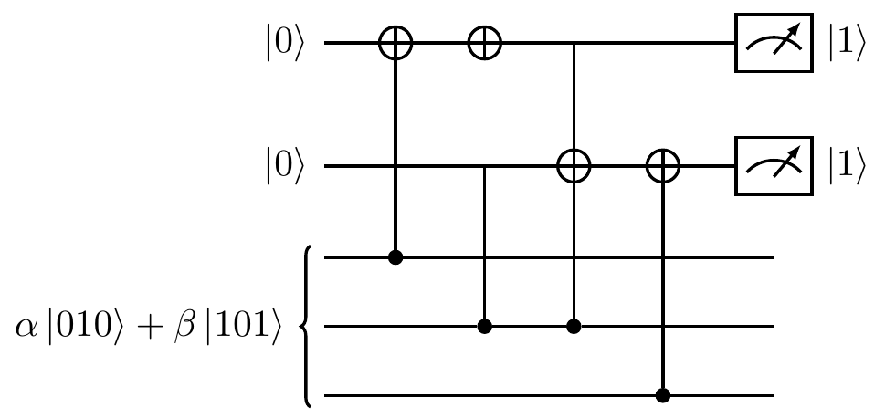
This decoding circuit is exactly the same as the ones for measuring the Pauli stabilisers ZZ\mathbf{1} and \mathbf{1}ZZ (as described in Section 7.4).
Measuring the two ancilla qubits gives us what is known as the error syndrome (or sometimes just syndrome, for short), which tells us how to correct the three qubits (known as the data qubits) of the code.
The theory behind this works as follows:
- if the first and second (counting from the top) data qubits are in the same state then the first ancilla will be in the |0\rangle state; otherwise the first ancilla will be in the |1\rangle state
- if the second and third data qubits are in the same state then the second ancilla will be in the |0\rangle state; otherwise the second ancilla will be in the |1\rangle state.
So the four possible error syndromes each indicate a different scenario:
- |00\rangle: no error
- |01\rangle: bit-flip in the first data qubit
- |10\rangle: bit-flip in the second data qubit
- |11\rangle: bit-flip in the third data qubit.
In our example, the error syndrome is |11\rangle, and so we know that the first and second qubits differ, as do the second and third.
This means that the first and third must be the same, and the second suffered the bit-flip error.
Knowing the error, we can now fix it by applying an X gate to the second qubit.
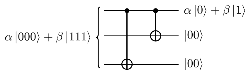
The final result is the state \alpha|000\rangle+\beta|111\rangle, which is then turned into (\alpha|0\rangle+\beta|1\rangle)|00\rangle by running the mirror image of the encoding circuit:
It is also important to note that the actual error correction can be implemented by a single unitary operation U_c on the five total qubits, with
\begin{aligned}
U_c
&= \big(|0\rangle\langle 0|\otimes|0\rangle\langle 0|\big)\otimes(\mathbf{1}\mathbf{1}\mathbf{1})
\\&+ \big(|0\rangle\langle 0|\otimes|1\rangle\langle 1|\big)\otimes(\mathbf{1}\mathbf{1}X)
\\&+ \big(|1\rangle\langle 1|\otimes|0\rangle\langle 0|\big)\otimes(X\mathbf{1}\mathbf{1})
\\&+ \big(|1\rangle\langle 1|\otimes|1\rangle\langle 1|\big)\otimes(\mathbf{1}X\mathbf{1}).
\end{aligned}
We draw the general circuit for bit-flip protection in Figure 13.7, writing out this U_c in full, denoting the error-syndrome measurement by a,b.
It is useful to represent syndrome measurements in terms of stabilisers.
For example, a computational basis measurement is represented by the Pauli Z operator.
The parity of two qubits is represented by the observable Z\otimes Z, since the Z\otimes Z measurement will have outcome +1 in the case of even parity and -1 in the case of odd parity (when applied to two of the three qubits).
To detect errors in a repetition encoding, we consider the parity of all pairs of qubits in the code; in the case of the three-qubit repetition code, we use the operators
\begin{gathered}
Z\otimes Z\otimes\mathbf{1}
Z\otimes \mathbf{1}\otimes Z
\mathbf{1}\otimes Z\otimes Z.
\end{gathered}
However, since Z^2=\mathbf{1}, it actually suffices to use only two of these, say Z\otimes Z\otimes\mathbf{1} and \mathbf{1}\otimes Z\otimes Z, because we can recover the last one as their product.
But these two operators are exactly generators of the stabiliser group
\mathcal{S}
= \{\mathbf{1}\mathbf{1}\mathbf{1}, ZZ\mathbf{1}, Z\mathbf{1}Z, \mathbf{1}ZZ\}
(where we again drop the tensor product symbol).
So, in summary, measuring the two generators of this stabiliser group gives us the error syndrome.
We can compile all the error syndromes (in the case of a single bit-flip) into a table:
| \mathbf{1}\mathbf{1}\mathbf{1} |
+ |
+ |
+ |
| X\mathbf{1}\mathbf{1} |
- |
- |
+ |
| \mathbf{1}X\mathbf{1} |
- |
+ |
- |
| \mathbf{1}\mathbf{1}X |
+ |
- |
- |
Here the rows are labelled by bit-flip errors, and the columns by the parity-check observables; we write \pm to mean \pm1.
Note how the + and - results correspond to the binary labels 0 and 1, and also how the Z\mathbf{1}Z column is simply given by the product of the other two measurement columns.
![The quantised version of the classical [3,1,3] code. If at most one bit-flip error occurs in the shaded region (which denotes the part where we transmit over a noisy channel), then this circuit perfectly corrects it, resulting in the successful transmission of the state \alpha|0\rangle+\beta|1\rangle.](qubit_guide_files/figure-html/single-bit-flip-complete-circuit-1.png)