14.5 … and error families

The quotient group²⁹⁷ N(\mathcal{S})/\mathcal{S} gave us logical operators, so the next thing to ask is what we get from the quotient group \mathcal{P}_n/N(\mathcal{S}).

The cosets of N(\mathcal{S}) inside \mathcal{P}_n are error families on the codespace V_\mathcal{S}. The individual elements of any error family (i.e. the elements of \mathcal{P}_n) are called physical errors.

Again, we can write \mathcal{P}_3 in such a way that we can immediately read off the cosets: \mathcal{P}_3 = \{\mathbf{1}, X\mathbf{1}\mathbf{1}, \mathbf{1}X\mathbf{1}, \mathbf{1}\mathbf{1}X\} \times N(\mathcal{S}) \times \{\pm1,\pm i\}. Ignoring the phases, the three (non-trivial) error families are single bit-flips:²⁹⁸ [X\mathbf{1}\mathbf{1}], [\mathbf{1}X\mathbf{1}], and [\mathbf{1}\mathbf{1}X]; these error families X_i map the codespace \mathcal{C} to the subspace \mathcal{C}_i, as shown in Figure 14.6.

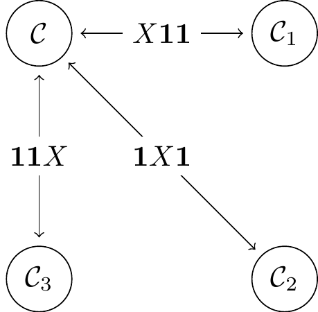
Figure 14.6: The single bit-flip error family X_i maps the codespace \mathcal{C} to the subspace \mathcal{C}_i, e.g. X_2|000\rangle=|010\rangle\in\mathcal{C}_2.

These errors also let us understand how the structure of the codespace is mirrored across each of the cosets. In other words, we picked \mathcal{C} to be our codespace, but what if we had instead picked \mathcal{C}_1? Well, we would get exactly the same code, just expressed in a different way, and this “different way” is described entirely by the error family [X\mathbf{1}\mathbf{1}]. What we mean by this is the following:²⁹⁹

• We can write \mathcal{C}_1 as the stabiliser space of \mathcal{S} conjugated by X\mathbf{1}\mathbf{1}, i.e. \begin{aligned} (X\mathbf{1}\mathbf{1})\langle ZZ\mathbf{1}, \mathbf{1}ZZ \rangle(X\mathbf{1}\mathbf{1})^{-1} &= \langle (X\mathbf{1}\mathbf{1})(ZZ\mathbf{1})(X\mathbf{1}\mathbf{1})^{-1}, (X\mathbf{1}\mathbf{1})(\mathbf{1}ZZ)(X\mathbf{1}\mathbf{1})^{-1} \rangle \\&= \langle -ZZ\mathbf{1}, \mathbf{1}ZZ \rangle \end{aligned} and, indeed, |100\rangle and |011\rangle are both stabilised by this group.
• The logical states of \mathcal{C}_1 are, by definition as our chosen basis, the elements |100\rangle and |011\rangle, but note that these are exactly the images of the logical states of \mathcal{C} under the error X\mathbf{1}\mathbf{1}, i.e. \begin{aligned} |0\rangle_{L,1} &\coloneqq |100\rangle = X\mathbf{1}\mathbf{1}|000\rangle \\|1\rangle_{L,1} &\coloneqq |011\rangle = X\mathbf{1}\mathbf{1}|111\rangle \end{aligned}
• The logical operators on \mathcal{C}_1 are the logical operators on \mathcal{C} conjugated by X\mathbf{1}\mathbf{1}, i.e \begin{aligned} X_{L,1} &\coloneqq (X\mathbf{1}\mathbf{1})(XXX)(X\mathbf{1}\mathbf{1})^{-1} \\&= XXX \\Z_{L,1} &\coloneqq (X\mathbf{1}\mathbf{1})(ZZZ)(X\mathbf{1}\mathbf{1})^{-1} \\&= -ZZZ \end{aligned} and, indeed, X_{L,1} and Z_{L,1} behave as expected on the new logical states, i.e. \begin{aligned} X_{L,1}\colon |0\rangle_{L,1} &\longmapsto |1\rangle_{L,1} \\|1\rangle_{L,1} &\longmapsto |0\rangle_{L,1} \\Z_{L,1}\colon |0\rangle_{L,1} &\longmapsto |0\rangle_{L,1} \\|1\rangle_{L,1} &\longmapsto -|1\rangle_{L,1} \end{aligned} as you can check by hand.

All in all, the chain of normal subgroups \mathcal{S} \triangleleft N(\mathcal{S}) \triangleleft \mathcal{P}_n really does describe the full structure of the code: logical states, logical operators, and error families.

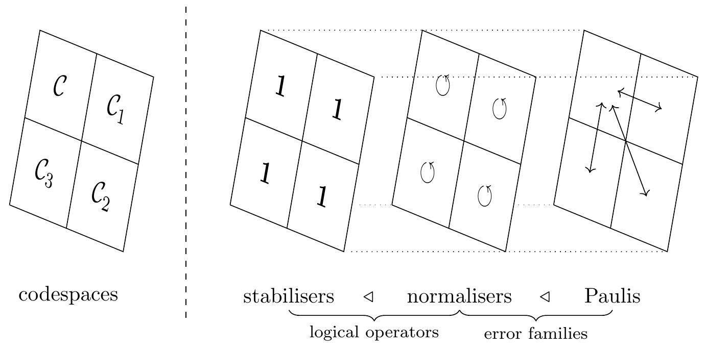
Figure 14.7: A visualisation of how the stabilisers, normalisers, and arbitrary Pauli operators act on the codespace decomposition: stabilisers act as the identity, normalisers move each subspace around within itself, and Pauli operators swap subspaces around between one another.

But this stabiliser formalism introduces some new ambiguity. In Section 14.3, we saw how measuring the three ancilla qubits in the Hamming [7,4,3] code gave us an error syndrome that we could use to determine on which qubit a Z-error had occurred, and back in Section 13.7 we saw the analogous error-syndrome setup for the three-qubit code. However, the stabiliser formalism is much more general: it makes no assumptions that only single-qubit errors can occur. This means that error syndromes will now only tell us which error family has occurred, not which specific physical error like they did before. At first, this seems like a definite downgrade from our previous theory — the actual errors that affect our circuits are still the physical errors, but now we have no way of knowing which one occurred, only which family it lives in! How are we to pick which coset representative to apply in order to correct the error?

As you might expect, the story is not yet over. Depending on the specifics of the scenario, sometimes knowing the error family is enough to be able to correct not just one physical error, but many. In order to give a more precise explanation, we need to take a step back and look at the scenarios that we’re actually trying to model — we do this in Section 14.7.

---

297. Recall that the elements of the quotient group G/H are exactly the cosets of H\triangleleft G.↩︎

298. We sometimes denote the coset P\cdot N(\mathcal{S}) simply by [P], just to save space.↩︎

299. Recall that conjugation expresses a change of basis: given an invertible (n\times n) matrix B, we can turn a basis \{v_1,\ldots,v_n\} into a new basis \{Bv_1,\ldots,Bv_n\}, and to write any operator A in this new basis we simply calculate BAB^{-1} (“undo the change of basis, apply A, then redo the change of basis”).↩︎