Encoding circuits
The previous sections have set up a lot of abstract theory about stabiliser codes, so now let’s take some time to look at more concrete aspects, such as the quantum circuits that actually let us build these codes “in practice”.
At the end of Section 14.3 we showed that the CSS construction could be applied to the Hamming [7,4,3] code over itself to obtain the so-called Steane [[7,1,3]] code, which has generators G_1,\ldots,G_6 given by the rows in the matrix
\begin{bmatrix}
X & X & \mathbf{1}& X & X & \mathbf{1}& \mathbf{1}
\\X & \mathbf{1}& X & X & \mathbf{1}& X & \mathbf{1}
\\\mathbf{1}& X & X & X & \mathbf{1}& \mathbf{1}& X
\\Z & Z & \mathbf{1}& Z & Z & \mathbf{1}& \mathbf{1}
\\Z & \mathbf{1}& Z & Z & \mathbf{1}& Z & \mathbf{1}
\\\mathbf{1}& Z & Z & Z & \mathbf{1}& \mathbf{1}& Z
\end{bmatrix}
and codespace given by the corresponding stabiliser space \mathcal{C}=V_\mathcal{S}, where \mathcal{S}=\langle G_1,\ldots,G_6\rangle.
Now, what are the logical states for this code?
Well, by definition they should be basis states for the stabiliser space V_{\langle G_1,\ldots,G_6\rangle}, but the “real” motivation for them is that they should just be the encodings of |0\rangle and |1\rangle in the code.
So the question becomes just how do we actually encode states with a code described by the stabiliser formalism?
But it turns out that we have already secretly answered this question in Exercise 7.8.5: the projector onto the \pm1-eigenspace of any G_i is given by \frac{1}{2}(\mathbf{1}\pm G_i).
Given stabiliser generators G_1,\ldots,G_s, the projector onto the stabiliser space V_{\langle G_1,\ldots,G_n\rangle} (i.e. the encoding for the corresponding stabiliser code) is given by
\prod_{i=1}^s \frac{1}{2}(\mathbf{1}+G_i).
In other words, we want to define
|0\rangle_L
\coloneqq \frac{1}{2^6} \left(\prod_{i=1}^6 (\mathbf{1}+G_i)\right) |0\rangle^{\otimes7}
since this will be in the +1-eigenspace of all of the G_i, which is exactly the stabiliser space V_{\langle G_1,\ldots,G_6\rangle}.
Similarly, we set
|1\rangle_L
\coloneqq \frac{1}{2^6} \left(\prod_{i=1}^6 (\mathbf{1}+G_i)\right) |1\rangle^{\otimes7}.
One thing to note is that the order of the product over the G_i doesn’t matter here: by design, every stabiliser generator commutes with every other, since they “overlap” (i.e. have non-identity terms) in an even number of positions, so any -1 signs arising from anticommutativity will cancel out with one another.
So for |0\rangle_L, when we expand out the product \prod_i(\mathbf{1}+G_i), we can simply move all the Z-type terms to the right and then forget them, since Z acts trivially on |0\rangle.
This means that we’re left with only the X-type terms, and there are eight of these:
\begin{aligned}
|0\rangle_L
\coloneqq \frac{1}{\sqrt{2^3}} \big(
& \mathbf{1}+ G_1 + G_2 + G_3
\\+& G_1G_2 + G_1G_3 + G_2G_3 + G_1G_2G_3
\big) |0000000\rangle
\\= \frac{1}{\sqrt{8}} \big(
&|0000000\rangle + |1101100\rangle + |1011010\rangle + |0111001\rangle
\\+&|0110110\rangle + |1010101\rangle + |1100011\rangle + |0001111\rangle
\big).
\end{aligned}
You can check by hand that this superposition is indeed invariant under each of the G_i.
Now, we could perform a similar calculation for |1\rangle_L, but since we have a CSS code we already know that X_L=X^{\otimes7} is an implementation for the logical X operator, so we can simply use this:
\begin{aligned}
|1\rangle_L
&\coloneqq X_L|0\rangle_L
\\&= \frac{1}{\sqrt{8}} \big(
|1111111\rangle + |0010011\rangle + |0100101\rangle + |1000110\rangle
\\&\phantom{\frac{1}{\sqrt{8}}\big(}
+|1001001\rangle + |0101010\rangle + |0011100\rangle + |1110000\rangle
\big).
\end{aligned}
We know what the logical states are, and by the previous discussions we also know what the logical operators are: cosets of \langle G_1,\ldots,G_6\rangle within its stabiliser in \mathcal{P}_7.
For example, not only is X^{\otimes7} an implementation of X_L, but so too is \mathbf{1}\mathbf{1}X\mathbf{1}\mathbf{1}XX.
So how can we actually access these logical states in order to do computation with them?
In other words, we need to design an encoding circuit that allows us to prepare the states |0\rangle_L and |1\rangle_L so that we can then perform computation on them.
As above, we will be able to neglect the Z-type stabilisers, because we’re working in the computational basis.
More specifically, since |0\rangle and |1\rangle live in the \pm1-eigenspace for Z, we don’t need to further project them to the stabiliser spaces of the Z-type stabilisers; we start with a basis in the stabiliser space for \pm Z, and when we encode we obtain a basis in the stabiliser space for \mathcal{S} and \pm Z_L.
This sort of duality always happens for CSS codes, and note that the choice of X versus Z isn’t “special” — if we switch to the |\pm\rangle basis then it would suffice to measure Z-type stabilisers, since we are already in the \pm1-eigenspace for X.
If this seems confusing, then don’t worry: look at the circuits below, follow the evolution of the input state through them, and then see what would happen if you did the same thing after adding the gates for the three missing Z-type stabilisers as well.
You will see that (up to a possible global phase) nothing changes.
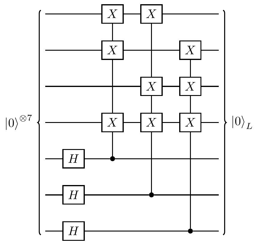
Inspired by the classical Hamming [7,4,3] code, we can think of the last three qubits in our seven-qubit encoding as the parity-check qubits, and read off the layout of the circuit from the parity-check matrix: the (3\times3) identity submatrix corresponds to the controls.
This gives us the encoding circuit in Figure 14.10.