9.7 Composition of quantum channels
We mentioned that quantum channels are combinations of
- adding a physical system in a fixed state (via tensoring),
- unitary transformations, and
- discarding a physical system (taking a partial trace).
As expected from the fact that the Stinespring point of view is equivalent to the Kraus point of view, each of these operations admits an operator-sum decomposition.
This is obvious for unitary evolution (
Adding a system. Any quantum system can be expanded by bringing in an auxiliary system in a fixed state
|a\rangle . This transformation takes vectors in the Hilbert space associated with the original system and tensors them with a fixed vector|a\rangle in the Hilbert space associated with the auxiliary system:|\psi\rangle \longmapsto |a\rangle\otimes|\psi\rangle = (|a\rangle\otimes\mathbf{1}) |\psi\rangle. In terms of density operators, we write this “expansion” transformation as\begin{aligned} \rho \longmapsto \rho' &= |a\rangle\langle a|\otimes\rho \\&= (|a\rangle\otimes\mathbf{1})\rho (\langle a|\otimes\mathbf{1}) \\&= V\rho V^\dagger \end{aligned} whereV=|a\rangle\otimes\mathbf{1} . We note thatV^\dagger V=\langle a|a\rangle\otimes\mathbf{1}=\mathbf{1} is the identity in the Hilbert space associated with the system, and soV is an isometry. Indeed, this transformation is an isometric embedding.Discarding a system. Conversely, given a composite system in state
\rho , we can discard one of its subsystems. The partial trace over an auxiliary system can be written in the Kraus representation as\begin{aligned} \rho \longmapsto \rho' &= \operatorname{tr}_\mathcal{A}\rho \\&= (\operatorname{tr}\otimes\mathbf{1})\rho \\&= \sum_i (\langle i|\otimes\mathbf{1})\rho(|i\rangle\otimes\mathbf{1}) \\&= \sum_i E_i\rho E^\dagger_i \end{aligned} where the vectors|i\rangle form an orthonormal basis in the Hilbert space associated with the auxiliary system. Again, we can check that the Kraus operatorsE_i=|i\rangle\otimes\mathbf{1} satisfy the completeness relation\sum_i E^\dagger_i E_i =\mathbf{1}\otimes\mathbf{1} (using the fact that\sum_i|i\rangle\langle i|=\mathbf{1} ).
Any sequential composition of two quantum channels
You might wonder why we explicitly called the above composition “sequential” — isn’t this how we always compose functions?
In actual fact, since we have access to tensor products, there is another sort of composition, namely parallel184 composition: if we have systems
Now that we know how to compose quantum channels in terms of Kraus operators, we can see that the Stinespring representation is perfectly consistent with the Kraus representation: the three basic operations that we are allowed to use to build channels in the Stinespring representation (i.e. adding a system, unitary evolution, and discarding a system) are all themselves quantum channels, in that they admit a Kraus decomposition.
Before moving on, we make a small (but important) remark:
When we compose quantum channels, each channel needs its own independent ancilla — do not share ancillas between different channels.
For example, say we have three channels,
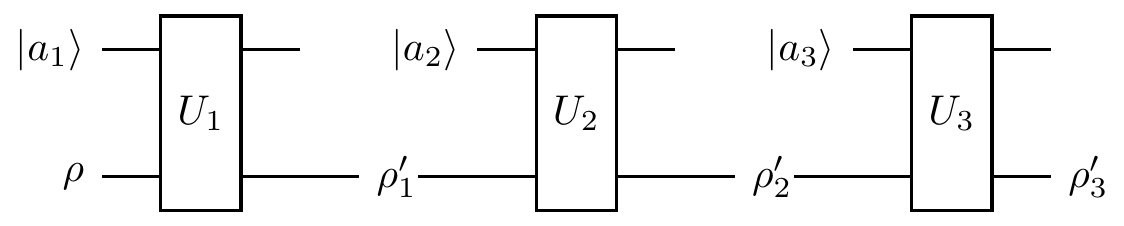
where each
Here we have tacitly assumed that the dimensions agree, i.e. that the output of
\mathcal{E} and the input of\mathcal{F} are of the same dimension, so that the composition makes sense.↩︎You might also call this simultaneous composition, to contrast with sequential composition, but “parallel” is by far the most commonly accepted terminology.↩︎