Composing quantum operations
In order to understand something in its full complexity it is always good to start with the simplest case.
Let us take a closer look at quantum interference in the simplest possible computing machine: the one that has only two distinguishable configurations — two quantum states — which we label as |0\rangle and |1\rangle.
We prepare the machine in some input state, usually |0\rangle, and let it evolve: the machine undergoes a prescribed sequence of computational steps, each of which induces transitions between the two “computational states” |0\rangle and |1\rangle.
The machine then ends in the output state |\psi\rangle=\alpha_0|0\rangle+\alpha_1|1\rangle, meaning the two outputs, |0\rangle and |1\rangle, are reached with probability amplitudes \alpha_0 and \alpha_1, respectively.
In the process of computation each computational step U (also referred to as an operation) sends state |k\rangle to state |l\rangle, where k,l=0,1, but only with some amplitude U_{lk}.
We write this as
|k\rangle \longmapsto \sum_l U_{lk} |l\rangle.
(watch out for the order of the indices).
In words, the state |k\rangle evolves into the specific state |l\rangle with probability amplitude U_{lk} and probability |U_{lk}|^2, so the whole situation is described by the superposition (i.e. the sum) of all of these.
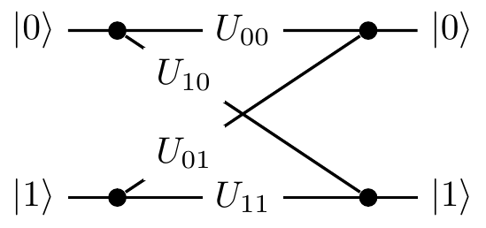
Thus any computational step U of this machine can be described by a matrix which tabulates all the transition amplitudes:
U =
\begin{bmatrix}
U_{00} & U_{01}
\\U_{10} & U_{11}
\end{bmatrix}.
The matrix element U_{lk} represents the amplitude of transition from state |k\rangle to state |l\rangle (again, watch the order of indices).
To be clear, the entries in this matrix are not any random complex numbers: their moduli squared represent transition probabilities, which in turn implies that such matrices must be unitary.
We can also describe U by drawing a diagram, which contains exactly the same information as the matrix representation, but just in a different form:

Now how can we find some quantum interference to study?
Consider two computational steps, U and V.
What is the amplitude that input |k\rangle will generate output |m\rangle?
We have to check all computational paths leading from input |k\rangle to output |m\rangle and add the corresponding amplitudes.
For example, as you can see in Figure 2.1, input |0\rangle and output |1\rangle are connected by the two computational paths: |0\rangle\mapsto|0\rangle\mapsto|1\rangle (amplitude V_{10}U_{00}) and |0\rangle\mapsto|1\rangle\mapsto|1\rangle (amplitude V_{11}U_{10}).
Thus the total amplitude that input |0\rangle gives output |1\rangle is the sum V_{10}U_{00}+V_{11}U_{10}, and when we take the modulus squared of this expression we will see the interference term.
In general, given U and V
\begin{aligned}
|k\rangle
&\longmapsto
\sum_l U_{lk}|l\rangle
\\|l\rangle
&\longmapsto
\sum_m V_{ml}|m\rangle
\end{aligned}
we can compose the two operations: we first apply U, and then V, to obtain
\begin{aligned}
|k\rangle
&\longmapsto
\sum_l U_{lk} \left(
\sum_m V_{ml}|m\rangle
\right)
\\&=
\sum_m \left(
\sum_l V_{ml}U_{lk}
\right) |m\rangle
\\&=
\sum_m (VU)_{mk} |m\rangle.
\end{aligned}
If you want to hone your quantum intuition think about it the following way.
The amplitude that input |k\rangle evolves to |m\rangle via a specific intermediate state |l\rangle is given by V_{ml}U_{lk} (evolutions are independent so the amplitudes are multiplied).
This done, we have to sum over all possible values of l (the transition can occur in several mutually exclusive ways so the amplitudes are added) to obtain \sum_l V_{ml}U_{lk}.
Thus the matrix multiplication VU (watch the order of matrices) in one swoop takes care of the multiplication and addition of amplitudes corresponding to different computational paths.

