Recoherence
If we could measure the environment in the |e_i\rangle basis without forgetting the result, then we would know what kind of error had occurred (say, some E_k) and could then simply restore the original state |\psi\rangle by reversing the action of E_k.
But the challenge lies in our lack of control over the environment.
At first glance, once our bunch of qubits, initially in state |\psi\rangle, gets entangled with the environment
|\psi\rangle|e\rangle
\longmapsto \sum_i E_i|\psi\rangle|e_i\rangle
the situation looks rather hopeless — we do not have any control over the environment.
However, there is a way around this.
We can couple the qubits to an auxiliary system that we do control (an ancilla), and then attempt to transfer the qubits–environment entanglement to a qubits–ancilla entanglement.
In other words, we prepare the ancilla in some prescribed state |a\rangle and try to undo the decoherence \mathcal{E} using some recovery or recoherence operator \mathcal{R} that acts as
|\psi\rangle|a\rangle
\longmapsto \sum_k R_k|\psi\rangle|a_k\rangle.
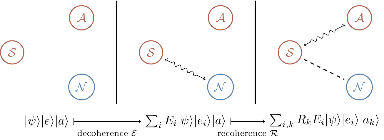
Thus decoherence followed by recoherence acts as
\begin{aligned}
\mathcal{R}\mathcal{E}\colon
|\psi\rangle|e\rangle|a\rangle
&\longmapsto \sum_i E_i|\psi\rangle|e_i\rangle|a\rangle
\\&\longmapsto \sum_{i,k} R_kE_i |\psi\rangle|e_i\rangle|a_k\rangle
\end{aligned}
which we can also express in a diagram, as in Figure 13.3.
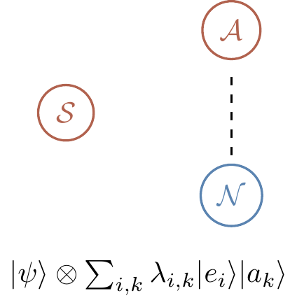
But for this to help us, we need to end up with in a state where the ancilla and the environment are entangled with one another, and the qubit is entangled with nothing, i.e. a state of the form
|\psi\rangle\otimes(\text{some entangled state of the ancilla and environment})
as shown in Figure 13.4
Ideally we would like this to hold for all states |\psi\rangle, but this turns out to be too much to ask: as we shall see in a moment, we will have to confine our recoverable states to those that belong to a subspace called the codespace.
But then at least for these states we expect to have
\sum_{i,k} R_kE_i |\psi\rangle|e_i\rangle|a_k\rangle
= \sum_{i,k} |\psi\rangle\otimes\lambda_{ik}|e_i\rangle|a_k\rangle.
The ability of R_k to perform the correction like this means that
R_kE_i
= \lambda_{ik}\mathbf{1}
when acting on the codespace states |\psi\rangle.
In turn, this means that
\begin{aligned}
\sum_k (R_k E_j)^\dagger(R_k E_i)
&= E_j^\dagger \left(\sum_k R_k^\dagger R_k\right) E_i
\\&= E_j^\dagger E_i
\\&= \lambda_{jk}^\star\lambda_{ik}\mathbf{1}
\end{aligned}
which reminds us of the hopefully now-familiar condition for being able to correct a randomly chosen isometry.
Last but not least, note that the recoherence operator \mathcal{R} not only allows us to recover from the errors E_i, but also from any errors that are in the linear span of these.
Thus if the errors E_i form a basis in the matrix space — as is the case for the Pauli matrices together with the identity — then once we design an error recovery scheme for the E_i, we will be able to correct any error.
If a quantum error correction method corrects errors E_1 and E_2, then it also corrects any linear combination of E_1 and E_2.
For example, in Section 13.2 we saw how the three-qubit encoding could correct for one of the possible errors \mathbf{1}, X_1, X_2, or X_3.
But not only can we correct for this discrete set of errors, we can also correct for any linear combination of them, such as R_{X_1}^(\theta), which acts as
|\psi\rangle
\overset{R_{X_1}(\theta)}{\longmapsto} \cos\frac{\theta}{2}|\psi\rangle + i\sin\frac{\theta}{2}X_1|\psi\rangle.
In other words, the scenario where, with probability \cos^2\frac{\theta}{2} we find that no error occurred, and with probability \sin^2\frac{\theta}{2} we find that the error X_1 occurred and correct it.