9.1 Everything is (secretly) unitary

At the fundamental level — and this should be your quantum mantra¹⁷⁰ — there is only unitary evolution, and if there is any other evolution then it has to be derived from a unitary evolution. From this perspective, any non-unitary evolution of an open system is induced by a unitary evolution of a larger system — all evolutions become unitary when you make your system large enough! But how? The short answer is: by adding (via tensoring) and removing (via partial trace) physical systems. A typical combination of these operations is shown in the following diagram:

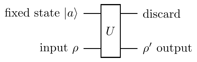
Let’s explain what this diagram is really saying.

First, as always, we prepare our system of interest in an input state \rho.

Next we dilate the system by “adding” (or “taking into account”) an auxiliary system¹⁷¹ which is large enough to include everything our system will interact with, and also large enough to be in a pure state |a\rangle. Mathematically, we do this by tensoring the input state \rho with |a\rangle\langle a| to obtain |a\rangle\langle a|\otimes\rho (here we place the auxiliary system first and our system of interest second). Importantly, we assume that we have “added in” a large enough auxiliary system that the resulting dilated system is closed, and thus undergoes unitary evolution, described by some U, resulting in the state U(|a\rangle\langle a|\otimes\rho)U^\dagger.

Finally, after all the (unitary) interactions have taken place, we trace out the auxiliary system, turning the joint state U(|a\rangle\langle a|\otimes\rho)U^\dagger of the dilated system into the final state of our system of interest: the output state \rho'.

We shall later show that the net effect of these three operations (adding, unitary evolution, and tracing out) can be written, as long as the initial state |a\rangle of the auxiliary system is not correlated with the input state \rho, in a nice compact way: \rho\longmapsto\rho' = \sum_i E_i\rho E_i^\dagger where the E_i are some operators that satisfy \sum_i E_i^\dagger E_i=\mathbf{1}. Such a linear map is called a completely positive trace-preserving map, or, in the parlance of quantum information science, a quantum channel.

We will elaborate on the mathematics behind quantum channels shortly, but for now let us only check the essential properties, i.e. that this map preserves both trace and positivity (as its name suggests).

Trace preserving. Since the trace is linear, invariant under cyclic permutations of operators, and we ask that \sum_i E_i^\dagger E_i=\mathbf{1}, we see that \operatorname{tr}\left(\sum_k E_k\rho E_k^\dagger\right) = \operatorname{tr}\left(\sum_k E^\dagger_k E_k \rho\right) = \operatorname{tr}\rho.
Positivity preserving. Since \rho is a positive¹⁷² (semi-definite) operator, so too is \sqrt{\rho}, and we thus see that \sum_k E_k\rho E_k^\dagger = \sum_k (E_k\sqrt{\rho})(\sqrt{\rho} E_k^\dagger).

These conditions are certainly necessary if we want to map density operators into legal density operators, but we shall see in a moment that they are not sufficient: quantum channels are not just positive maps, but instead completely positive maps.

We will discuss the special properties of completely positive trace preserving maps, describe the most common examples, and, last but not least, specify when the action of quantum channels can be reversed, or corrected, so that we can recover the original input state. This will set the stage for our subsequent discussion of quantum error correction.

…There is only unitary evolution. There is only unitary evolution. There is only unitary evolution… …and everything else is cheating.↩︎
Depending on the context, the auxiliary system is either called the ancilla (usually when we can control it) or the environment (usually when we cannot control it).↩︎
Recall that an operator is positive if and only if it can be written in the form XX^\dagger for some X (here X=E_k\sqrt{\rho}). Also, the sum of positive operators is again a positive operator.↩︎