1.5 Interferometers

One of the most fundamental family of experiments for our purposes are so-called interference experiments, modern versions of which are performed using internal degrees of freedom of atoms and ions. For example, Ramsey interferometry, named after American physicist Norman Ramsey (1915–2011), is a generic name for an interference experiment in which atoms are sent through two separate “resonant interaction” zones, known as Ramsey zones, separated by an intermediate “dispersive interaction” zone.

Many beautiful experiments of this type were carried out in the 1990s in Serge Haroche’s lab at the Ecole Normale Supérieure in Paris. Rubidium atoms were sent through two separate interaction zones (resonant interaction in the first and the third cavity) separated by a phase inducing dispersive interaction zone (the central cavity). The atoms were subsequently measured, via a selective ionisation, and found to be in one of the two preselected energy states, here labeled as |0\rangle and |1\rangle. The fraction of atoms found in states |0\rangle or |1\rangle showed a clear dependence on the phase shifts induced by the dispersive interaction in the central cavity. In 2012, Serge Haroche and Dave Wineland shared the Nobel Prize in physics for “ground-breaking experimental methods that enable measuring and manipulation of individual quantum systems.” Let us now try to understand what this experiment actually entails.

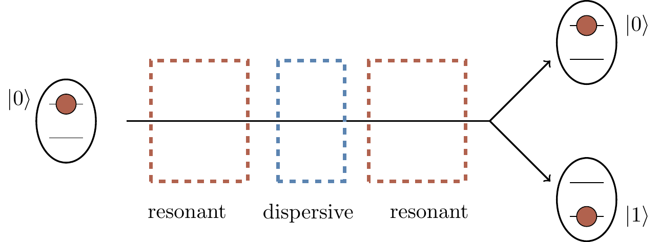
Figure 1.1: A schematic diagram of a Ramsey interference experiment.

The three rectangular boxes in Figure 1.1 represent three cavities, each cavity being an arrangement of mirrors which traps electromagnetic field (think about standing waves in between two mirrors). The oval shapes represent rubidium atoms with two preselected energy states²⁸ labelled as |0\rangle and |1\rangle. Each atom is initially prepared in a highly excited internal energy state |0\rangle and zips through the three cavities, from the left to the right. In each cavity the atom interacts with the cavity field. The first and the third cavities are, for all theoretical purposes, identical: their frequencies are tuned to the resonant frequency of the atom, and the atom exchanges energy with the cavity, going back and forth between its energy states |0\rangle and |1\rangle. In contrast, in the second (central) cavity, the atom undergoes the so-called dispersive interaction: it is too off-resonance for the atom to exchange energy with the field, but the atom’s energy states “feel” the field and acquire phase shifts. After experiencing this well timed sequence of resonant–dispersive–resonant interactions, the energy of the atom is measured and the atom is found to be either in state |0\rangle or state |1\rangle. The (surprising) result of this experiment is analogous to that of the double-slit experiment described above: the fraction of atoms found in state |0\rangle or |1\rangle shows a clear dependence on the phase shifts induced by the dispersive interaction in the central cavity.

We can understand this interference better if we follow the two internal states of the atom as it moves through the three cavities.

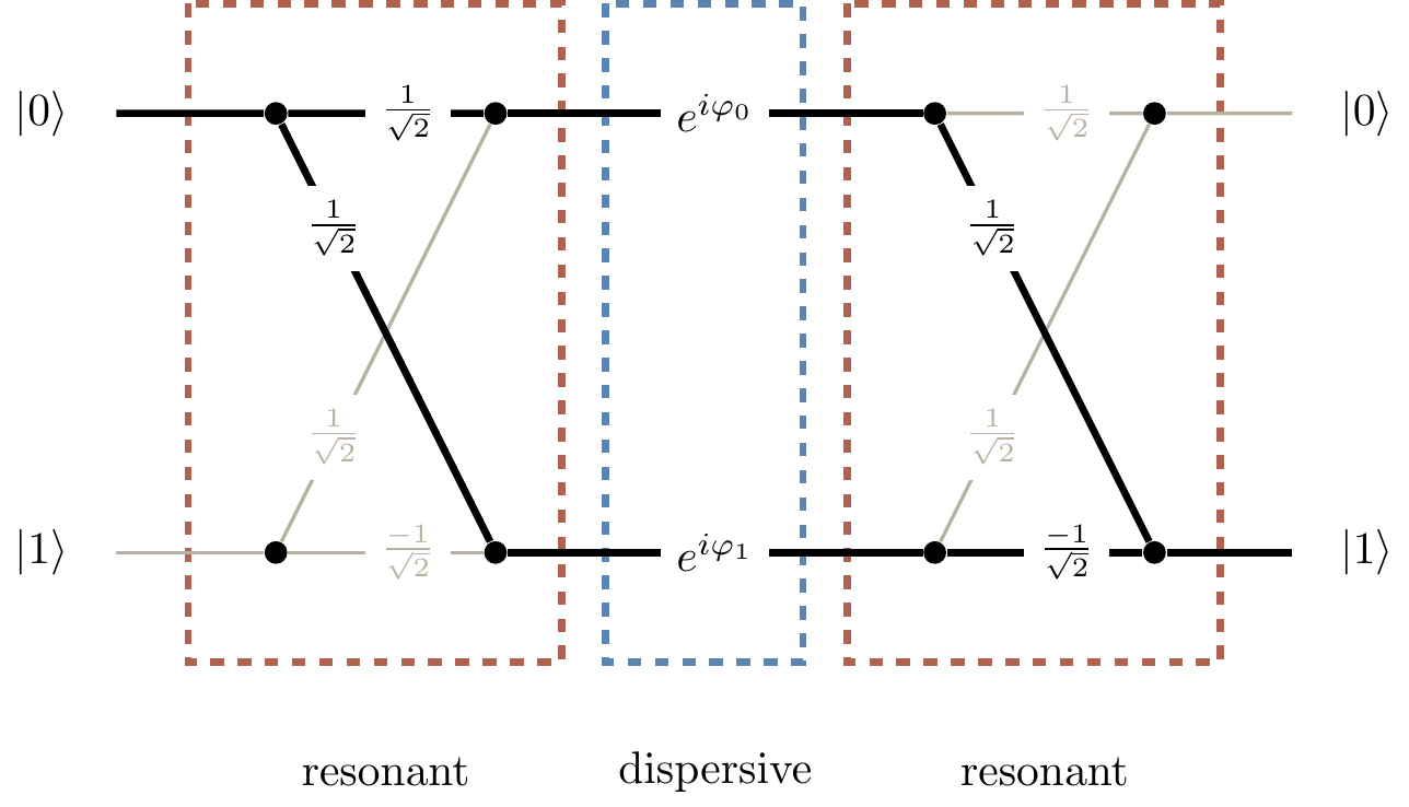
Figure 1.2: The Ramsey interferometer represented as an abstract diagram, to be read from left to right. The line segments represent transitions between the two states, |0\rangle and |1\rangle, and the numbers are the corresponding probability amplitudes.

Suppose we are interested in the probability that the atom, initially in state |0\rangle, will be found, after completing its journey through the three cavities, in state |1\rangle. As you can see in Figure 1.2, this can happen in two ways, as indicated by the two thick paths connecting the input state |0\rangle on the left with the output state |1\rangle on the right. Again, let U_{ij} denote the probability amplitude that input |j\rangle generates output |i\rangle (for i,j=0,1).

We can see from the diagram that \begin{aligned} U_{10} &= \frac{1}{\sqrt{2}} e^{i\varphi_0}\frac{1}{\sqrt{2}} + \frac{1}{\sqrt{2}} e^{i\varphi_1}\frac{-1}{\sqrt{2}} \\&= \frac{1}{2} \left(e^{i\varphi_0}-e^{i\varphi_1}\right). \end{aligned} Then, using the trick of writing x=\frac{x+y}{2}+\frac{x-y}{2} and y=\frac{x+y}{2}-\frac{x-y}{2}, followed by Euler’s formula (e^{i\alpha}=\cos\alpha+i\sin\alpha), we see that \begin{aligned} U_{10} &= \frac{1}{2} \left(e^{i\varphi_0}-e^{i\varphi_1}\right) \\&= \frac{1}{2}\left( e^{i\frac{\varphi_0+\varphi_1}{2}}e^{i\frac{\varphi_0-\varphi_1}{2}} - e^{i\frac{\varphi_0+\varphi_1}{2}}e^{-i\frac{\varphi_0-\varphi_1}{2}}\right) \\&= \frac{1}{2} e^{i\frac{\varphi_0+\varphi_1}{2}} \left( e^{i\frac{\varphi_0-\varphi_1}{2}} - e^{-i\frac{\varphi_0-\varphi_1}{2}}\right) \\&= \frac{1}{2} e^{i\frac{\varphi_0+\varphi_1}{2}} \left( 2i \sin\left(\frac{\varphi_0 - \varphi_1}{2}\right) \right) \\&= -ie^{i\frac{\varphi_0+\varphi_1}{2}}\sin\frac{\varphi_1-\varphi_0}{2} \end{aligned} where the relative phase \varphi=\varphi_1-\varphi_0 shows up yet again.

The corresponding probability (i.e. that an atom, initially in state |0\rangle, will be found in state |1\rangle) is then²⁹ \begin{aligned} P_{10} &= \vert U_{10}\vert^2 \\&= \left\vert -ie^{i\frac{\varphi_0+\varphi_1}{2}}\sin\frac{\varphi_1-\varphi_0}{2} \right\vert^2 \\&= \left\vert \sin\frac{\varphi_1-\varphi_0}{2} \right\vert^2 \\&= \frac{1}{2}(1 - \cos\varphi) \end{aligned} where we use the fact that |i|^2=1 and |e^{i\alpha}|^2=1 for any \alpha, along with the double angle formula \cos2\theta=1-2\sin^2\theta.

You should recognise the first term \frac{1}{2} as the “classical” probability and the second one -\frac{1}{2}\cos\varphi as the interference term. We can repeat such calculations for any other pair of input–output states. This approach works fine here but, in general, tracking all possible paths in evolving quantum systems can become messy when the number of input and output states increases. There is, however, a neat way of doing these calculations: matrix multiplication.

The effect of each interaction on atomic states can be described by a matrix of transition amplitudes, as illustrated in Figure 1.3, and then the sequence of independent interactions is described by the product of these matrices: we compile all the U_{ij} into one matrix U. \begin{aligned} U &= \begin{bmatrix} \frac{1}{\sqrt{2}} & \frac{1}{\sqrt{2}} \\\frac{1}{\sqrt{2}} & \frac{-1}{\sqrt{2}} \end{bmatrix} \begin{bmatrix} e^{i\varphi_0} & 0 \\0 & e^{i\varphi_1} \end{bmatrix} \begin{bmatrix} \frac{1}{\sqrt{2}} & \frac{1}{\sqrt{2}} \\\frac{1}{\sqrt{2}} & \frac{-1}{\sqrt{2}} \end{bmatrix} \\&= e^{i\frac{\varphi_0+\varphi_1}{2}} \begin{bmatrix} \cos\frac{\varphi}{2} & -i\sin\frac{\varphi}{2} \\\ -i\sin\frac{\varphi}{2}& \cos\frac{\varphi}{2} \end{bmatrix} \\&= \begin{bmatrix} U_{00} & U_{01} \\U_{10} & U_{11} \end{bmatrix} \end{aligned} where \varphi = \varphi_1-\varphi_0, as before.

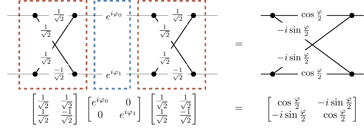
Figure 1.3: The Ramsey interferometer represented as an abstract diagram (matrix approach). Here we have omitted the |0\rangle and |1\rangle labels, just to simply the diagram. We also ignore (for reasons that we will later explain) the global phase factor of e^{i\frac{\varphi_0+\varphi_1}{2}}.

In general, quantum operation A followed by quantum operation B is the quantum operation described by the matrix product³⁰ BA. Indeed, the expression (BA)_{ij}=\sum_k B_{ik}A_{kj} is the sum over amplitudes that input |j\rangle generates output |i\rangle via a specific intermediate state |k\rangle. As you can see, the matrix approach is a wonderful bookkeeping tool: in one package it takes care of both multiplying and adding probability amplitudes corresponding to all the contributing paths.

---

28. If the language of energy states of atoms is unfamiliar to you, don’t worry! Here we are just trying to give some physical motivation for one of the fundamental quantum circuits which we will see pop up time and time again. Vaguely, though, you can just have in your mind the idea that atoms have a certain amount of energy at any given time, but the amount that they can have is one of a number of fixed amounts, depending on the chemistry of the atom. This is in fact one of the key principles in the history of quantum physics, and is the reason for the word “quantum”.↩︎

29. From the classical probability theory perspective the resonant interaction induces a random switch between |0\rangle and |1\rangle (why?) and the dispersive interaction has no effect on these two states (why?). One random switch followed by another random switch is exactly the same as a single random switch (if you flip a coin twice and just observe the last result, this is probabilistically the same as just flipping the coin once), which gives \frac{1}{2} for the probability that input |0\rangle becomes output |1\rangle.↩︎

30. Note the order of the matrices: the composition “A followed by B” is BA, not AB! This reflects the fact that, in linear algebra, we apply a matrix to a vector on the left, i.e. A applied to v is written Av.↩︎