1.11 Remarks and exercises

1.11.1 A historical remark

Back in 1926, Max Born simply postulated the connection between amplitudes and probabilities, but did not get it quite right on his first attempt. In the original paper⁴⁰ proposing the probability interpretation of the state vector (wavefunction) he wrote:

… If one translates this result into terms of particles only one interpretation is possible. $\Theta_{\eta,\tau,m}(\alpha,\beta,\gamma)$ [the wavefunction for the particular problem he is considering] gives the probability $^*$ for the electron arriving from the $z$ direction to be thrown out into the direction designated by the angles $\alpha,\beta,\gamma$ …

$^*$ Addition in proof: More careful considerations show that the probability is proportional to the square of the quantity $\Theta_{\eta,\tau,m}(\alpha,\beta,\gamma)$ .

1.11.2 Modifying the Born rule

Suppose that we modified the Born rule, so that probabilities were given by the absolute values of amplitudes raised to the power $p$ (for some $p>0$ not necessarily equal to $2$ ). Then physically admissible evolutions would still have to preserve the normalisation of probability: mathematically speaking, they would have to be isometries of $p$ -norms.

The $p$ -norm of a vector $v=(v_1, v_2,\ldots, v_n)$ , for $p\in\mathbb{N}$ , is defined as⁴¹ $\sqrt[{}^p]{|v_1|^p + |v_2|^p + \ldots + |v_n|^p}.$ It is clear that any permutation of vector components and multiplication by phase factors (i.e. unit complex numbers, of the form $e^{i\varphi}$ for some $\varphi$ ) will leave any $p$ -norm unchanged. It turns out that these complex permutations are the only isometries, except for one special case: $p=2$ . For $p=2$ , the isometries are exactly unitaries, which form a continuous group; in all other cases we are restricted to discrete permutations. We do not have to go into details of the proof since we can see this result.

$The unit spheres in the p-norm for p=1,2,42,\infty (where the definition of the \infty-norm is slightly different; we will come back to this in Section 12.11.2).$

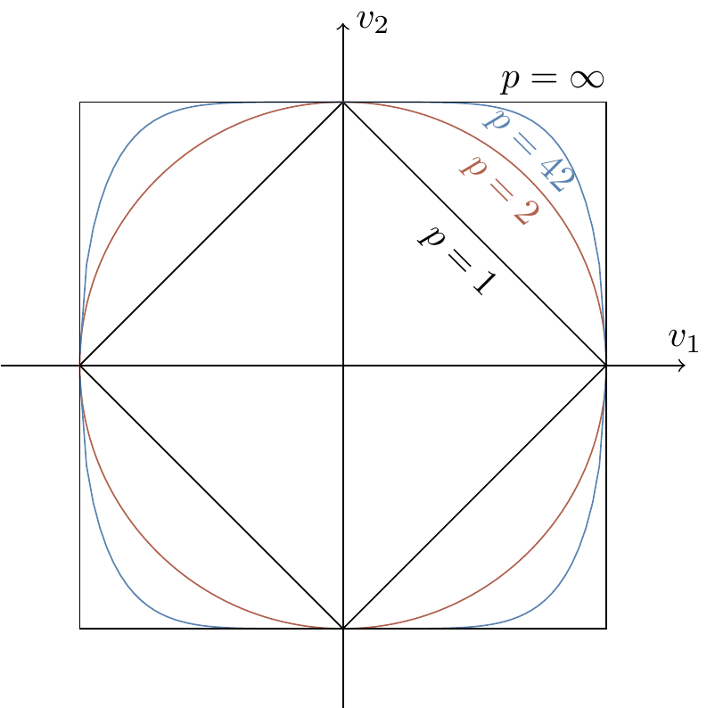
Figure 1.7: The unit spheres in the $p$ -norm for $p=1,2,42,\infty$ (where the definition of the $\infty$ -norm is slightly different; we will come back to this in Section 12.11.2).

The image of the unit sphere must be preserved under probability preserving operations. As we can see in Figure 1.7, the $2$ -norm is special because of its rotational invariance (it describes a circle) — the probability measure picks out no preferred basis in the space of state vectors. Moreover, it respects unitary operations and does not restrict them in any way. If the admissible physical evolutions were restricted to discrete symmetries, e.g. permutations, then there would be no continuity, and no concept of “time” as we know it.

1.11.3 Many computational paths

A quantum computer starts calculations in some initial state, then follows $n$ different computational paths which lead to the final output. The computational paths are followed with probability amplitudes $\frac{1}{n}e^{i k \varphi}$ , where $\varphi$ is a fixed angle $0< \varphi <2\pi$ and $k=0,1,...n-1$ . Using the fact that $1+z+z^2+\ldots + z^n= \frac{1-z^{n+1}}{1-z}$ , show that the probability $P$ of generating the output is given by $P = \frac{1}{n^2}\left\vert \frac{1-e^{i n\varphi}}{1-e^{i\varphi}} \right\vert^2 = \frac{1}{n^2} \frac{\sin^2 (n\frac{\varphi}{2})}{\sin^2 (\frac{\varphi}{2})}.$ for $0<\varphi<2\pi$ , and that $P=1$ when $\varphi=0$ . Plot the probability as a function of $\varphi$ .

1.11.4 Distant photon emitters

Imagine two distant stars, A and B, that emit identical photons. If you point a single detector towards them you will register a click every now and then, but you never know which star the photon came from. Now prepare two detectors and point them towards the stars. Assume the photons arrive with the probability amplitudes specified in Figure 1.8. Every now and then you will register a coincidence: the two detectors will both click.

Calculate the probability of such a coincidence.
Now assume that $z\approx \frac{1}{r}e^{i{2r\pi}/{\lambda}}$ , where $r$ is the distance between detectors and the stars and $\lambda$ is some fixed constant. How can we use this to measure $r$ ?

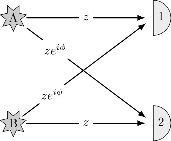
Figure 1.8: Two photon detectors pointing at two stars, with the probabilities of detection labelling the arrows.

1.11.5 Quantum Turing machines

The classical theory of computation is essentially the theory of the universal Turing machine — the most popular mathematical model of classical computation. Its significance relies on the fact that, given a possibly very large but still finite amount of time, the universal Turing machine is capable of any computation that can be done by any modern classical digital computer, no matter how powerful. The concept of Turing machines may be modified to incorporate quantum computation, but we will not follow this path. It is much easier to explain the essence of quantum computation talking about quantum logic gates and quantum Boolean networks or circuits. The two approaches are computationally equivalent, even though certain theoretical concepts, e.g. in computational complexity, are easier to formulate precisely using the Turing machine model. The main advantage of quantum circuits is that they relate far more directly to proposed experimental realisations of quantum computation.

1.11.6 More time, more memory

A quantum machine has $N$ perfectly distinguishable configurations. What is the maximum number of computational paths connecting a specific input with a specific output after $k$ steps of the machine?

Suppose you are using your laptop to add together amplitudes pertaining to each of the paths. As $k$ and $N$ increase you may need more time and more memory to complete the task. How does the execution time and the memory requirements grow with $k$ and $N$ ? In particular, which will be the thing that limits you sooner: not having enough memory, not having enough time, or both?

1.11.7 Asymptotic behaviour: big-O

In order to make qualitative distinctions between how different functions grow we will often use the asymptotic big- $\mathcal{O}$ notation. For example, suppose an algorithm running on input of size $n$ takes $a n^2+bn+c$ elementary steps, for some positive constants $a, b$ and $c$ . These constants depend mainly on the details of the implementation and the choice of elementary steps. What we really care about is that, for large $n$ , the whole expression is dominated by its quadratic term. We then say that the running time of this algorithm grows as $n^2$ , and we write it as $\mathcal{O}(n^2)$ , ignoring the less significant terms and the constant coefficients. More precisely, let $f(n)$ and $g(n)$ be functions from positive integers to positive reals. You may think of $f(n)$ and $g(n)$ as the running times of two algorithms on inputs of size $n$ . We say $f=\mathcal{O}(g)$ ,⁴² which means that $f$ grows no faster than $g$ , if there is a constant $c>0$ such that $f(n)\leqslant c g(n)$ for all sufficiently large values of $n$ . Essentially, $f=\mathcal{O}(g)$ is a very loose analogue of $f \leqslant g$ . In addition to the big- $\mathcal{O}$ notation, computer scientists often use $\Omega$ for lower bounds: $f=\Omega (g)$ means $g=\mathcal{O}(f)$ . Again, this is a very loose analogue of $f \geqslant g$ .

When we say that $f(n)=\mathcal{O}(\log n)$ , why don’t we have to specify the base of the logarithm?
Let $f(n)=5n^3+1000n+50$ . Is $f(n)=\mathcal{O}(n^3)$ , or $\mathcal{O}(n^4)$ , or both?
Which of the following statements are true?
1. $n^k=\mathcal{O}(2^n)$ for any constant $k$
2. $n!=\mathcal{O}(n^n)$
3. if $f_1=\mathcal{O}(g)$ and $f_2=\mathcal{O}(g)$ , then $f_1+f_2=\mathcal{O}(g)$ .

1.11.8 Polynomial is good, and exponential is bad

In computational complexity the basic distinction is between polynomial and exponential algorithms. Polynomial growth is good and exponential growth is bad, especially if you have to pay for it. There is an old story about the legendary inventor of chess who asked the Persian king to be paid only by a grain of cereal, doubled on each of the 64 squares of a chess board. The king placed one grain of rice on the first square, two on the second, four on the third, and he was supposed to keep on doubling until the board was full. The last square would then have $2^{63}=9,223,372,036,854,775,808$ grains of rice, more than has been ever harvested on planet Earth, to which we must add the grains of all previous squares, making the total number about twice as large. If we placed that many grains in an unbroken line we would reach the nearest star Alpha Centauri, our closest celestial neighbour beyond the solar system, about $4.4$ light-years away.⁴³

The moral of the story: if whatever you do requires an exponential use of resources, you are in trouble.

1.11.9 Imperfect prime tester

There exists a randomised algorithm which tests whether a given number $N$ is prime.⁴⁴ The algorithm always returns $\texttt{yes}$ when $N$ is prime, and the probability it returns $\texttt{yes}$ when $N$ is not prime is $\varepsilon$ , where $\varepsilon$ is never greater than a half (independently, each time you run the algorithm). You run this algorithm $r$ times (for the same value of $N$ ), and each time the algorithm returns $\texttt{yes}$ . What is the probability that $N$ is not prime?

1.11.10 Imperfect decision maker

Suppose a randomised algorithm solves a decision problem, returning $\texttt{yes}$ or $\texttt{no}$ answers. It gets the answer wrong with a probability not greater than $\frac{1}{2}-\delta$ , where $\delta>0$ is a constant.⁴⁵ If we are willing to accept a probability of error no larger than $\varepsilon$ , then it suffices to run the computation $r$ times, where $r=\mathcal{O}(\log 1/\varepsilon)$ .

If we perform this computation $r$ times, how many possible sequences of outcomes are there?
Give a bound on the probability of any particular sequence with $w$ wrong answers.
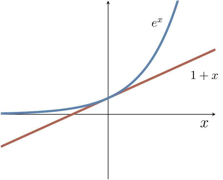
If we look at the set of $r$ outcomes, we will determine the final outcome by performing a majority vote. This can only go wrong if $w>r/2$ . Give an upper bound on the probability of any single sequence that would lead us to the wrong conclusion.
Using the bound $1-x\leqslant e^{-x}$ , conclude that the probability of our coming to the wrong conclusion is upper bounded by $e^{-2r\delta^2}$ .

Max Born, “Zur Quantenmechanik der Stoßvorgänge”, Zeitschrift für Physik 37 (1926), pp. 893–867.↩︎
In the case $p=2$ , we recover the usual Pythagorean/Euclidean equation that we all know and love: the distance of the point $(v_1,v_2,\ldots,v_n)$ from the origin is $\sqrt{v_1^2+v_2^2+\ldots+v_n^2}$ ; if we take $n=2$ as well then we recover the Pythagoras theorem.↩︎
$f=\mathcal{O}(g)$ is pronounced as “ $f$ is big-oh of $g$ ”.↩︎
One light year (the distance that light travels through a vacuum in one year) is $9.4607\times10^{15}$ metres.↩︎
Primality used to be given as the classic example of a problem in $\texttt{BPP}$ but not $\texttt{P}$ . However, in 2002 a deterministic polynomial time test for primality was proposed by Manindra Agrawal, Neeraj Kayal, and Nitin Saxena in the wonderfully titled paper “PRIMES is in $\texttt{P}$ ”. Thus, since 2002, primality has been in $\texttt{P}$ .↩︎
This result is known as the Chernoff bound.↩︎